Introduction
This page covers cylindrical coordinates. The initial part talks about the relationships between position, velocity, and acceleration. The second section quickly reviews the many vector calculus relationships.Rectangular and Cylindrical Coordinates
Rectangular and cylindrical coordinate systems are related by
\[ \begin{eqnarray} x & = & r \cos \theta \\ y & = & r \sin \theta \\ z & = & z \end{eqnarray} \]
and by
\[ \begin{eqnarray} r & = & \sqrt{ x^2 + y^2 } \\ \theta & = & Tan^{-1} \left( {y / x} \right) \\ z & = & z \end{eqnarray} \]
Cylindrical coordinates are "polar coordinates plus a z-axis."
Position, Velocity, Acceleration
The position of any point in a cylindrical coordinate system is written as\[ {\bf r} = r \; \hat{\bf r} + z \; \hat{\bf z} \]
where \(\hat {\bf r} = (\cos \theta, \sin \theta, 0)\). Note that \(\hat \theta\) is not needed in the specification of \({\bf r}\) because \(\theta\), and \(\hat{\bf r} = (\cos \theta, \sin \theta, 0)\) change as necessary to describe the position. However, it will appear in the velocity and acceleration equations because
\[ {\partial \, \hat{\bf r} \over \partial \, t} \; = \; {\partial \over \partial \, t} (\cos \theta, \sin \theta, 0) \; = \; (-\sin \theta, \cos \theta, 0) {\partial \, \theta \over \partial \, t} \; = \; \omega \, \hat{\boldsymbol{\theta}} \]
\[ {\partial \, \hat{\boldsymbol{\theta}} \over \partial \, t} \; = \; {\partial \over \partial \, t} (-\sin \theta, \cos \theta, 0) \; = \; (-\cos \theta, -\sin \theta, 0) {\partial \, \theta \over \partial \, t} \; = \; -\omega \, \hat{\bf r} \]
and finally \( {\partial \, \hat{\bf z} \over \partial \, t} \; = \; 0 \) because \(\hat{\bf z}\) does not change direction.
In summary, identities used here include
\[ \omega = {\partial \, \theta \over \partial \, t} \qquad \qquad \alpha = {\partial \, \omega \over \partial \, t} \qquad \qquad {\partial \, \hat{\bf r} \over \partial \, t} = \omega \, \hat{\boldsymbol{\theta}} \qquad \qquad {\partial \, \hat{\boldsymbol{\theta}} \over \partial \, t} = -\omega \, \hat{\bf r} \qquad \qquad {\partial \, \hat{\bf z} \over \partial \, t} \; = \; 0 \]
\[ {\bf v} \quad = \quad {\partial \over \partial \, t} (r \; \hat{\bf r} + z \; \hat{\bf z}) \quad = \quad (\dot r \, \hat{\bf r} + r \; \omega \; \hat{\boldsymbol{\theta}} + \dot z \, \hat{\bf z}) \]
This could also be written as
\[ {\bf v} = (v_r \, \hat{\bf r} + v_\theta \hat{\boldsymbol{\theta}} + v_z \, \hat{\bf z}) \]
where \(v_r = \dot r, v_\theta = r \, \omega,\) and \(v_z = \dot z\).
Differentiating again to get acceleration...
\[ \begin{eqnarray} {\bf a} & = & {\partial \over \partial \, t} (\dot r \, \hat{\bf r} + r \; \omega \; \hat{\boldsymbol{\theta}} + \dot z \, \hat{\bf z}) \\ \\ & = & \ddot r \hat{\bf r} + \dot r \, \omega \; \hat{\boldsymbol{\theta}} + \dot r \, \omega \; \hat{\boldsymbol{\theta}} + r \, \alpha \, \hat{\boldsymbol{\theta}} - r \, \omega^2 \, \hat{\bf r} + \ddot z \, \hat{\bf z} \\ \\ & = & ( \ddot r - r \, \omega^2 ) \, \hat{\bf r} + ( r \, \alpha + 2 \, \dot r \, \omega ) \; \hat{\boldsymbol{\theta}} + \ddot z \, \hat{\bf z} \end{eqnarray} \]
The \(- r \, \omega^2 \, \hat{\bf r}\) term is the centripetal acceleration. Since \( \omega = v_\theta / r \), the term can also be written as \(- (v^2_\theta / r) \, \hat{\bf r} \).
The \(2 \dot r \omega \, \hat{\boldsymbol{\theta}}\) term is the Coriolis acceleration. It can also be written as \(2 \, v_r \, \omega \, \hat{\boldsymbol{\theta}}\) or even as \( (2 \, v_r \, v_\theta / r ) \hat{\boldsymbol{\theta}}\), which stresses the product of \(v_r\) and \(v_\theta\) in the term.
Centripetal Accelerations in the Tire
The centripetal acceleration of a tire traveling at 70 mph is remarkably high. 70 mph is 31.3 m/s, and this is \(v_\theta\). For a tire with a 0.3 m radius, the centripetal acceleration is\[ {v^2_\theta \over r} \quad = \quad {\text{31.3 m/s}^2 \over \text{0.3 m}} \quad = \quad \text{3,270 m}^2\text{/s} \quad = \quad \text{333 g's} \]
Cylindrical Acceleration Example
This example uses the function, \(r=[17-\cos(4\theta)]/16\), with \(\theta = t\), and calculates acceleration components.The function looks like
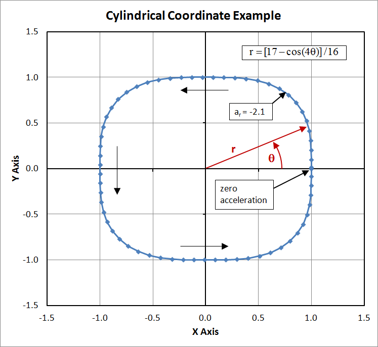
The derivatives of \(r\) are
\[ \begin{eqnarray} \dot r & = & {\partial \, r \over \partial \, t} = \left( {\partial \, r \over \partial \, \theta} \right) \left( {\partial \, \theta \over \partial \, t} \right) \\ \\ \\ & = & {1 \over 4} \sin(4 \theta) * \omega \qquad \text{where } \quad \omega = 1 \end{eqnarray} \]
and the 2nd derivative is
\[ \begin{eqnarray} \ddot r & = & \cos(4 \theta) \end{eqnarray} \]
So the acceleration vector is
\[ \begin{eqnarray} {\bf a} & = & ( \ddot r - r \, \omega^2 ) \, \hat{\bf r} + ( r \, \alpha + 2 \, \dot r \, \omega ) \; \hat{\boldsymbol{\theta}} + \ddot z \, \hat{\bf z} \\ \\ \\ & = & \left[ \cos(4 \theta) - {17 - \cos(4 \theta) \over 16 } \right] \hat{\bf r} + {1 \over 2} \sin(4 \theta) \hat{\boldsymbol{\theta}} \\ \\ \\ & = & { 17 \over 16} \left[ \cos(4 \theta) - 1 \right] \, \hat{\bf r} + {1 \over 2} \sin(4 \theta) \hat{\boldsymbol{\theta}} \end{eqnarray} \]
2nd Cylindrical Acceleration Example
A bar is rotating at a rate, \(\omega\). A collar starts at \(R_o\) and is being flung off with zero friction. So the radial acceleration is zero. Therefore
\[ a_r = \ddot r - r \, \omega^2 = 0 \]
This is a 2nd order differential equation, whose solution is
\[ r = A e^{\omega \, t} + B \, e^{-\omega \, t} \]
Assume the initial conditions are \(r(0) = R_o\) and \(\dot r(0) = 0\). This leads to
\[ R_o = A + B \] \[ \;\;\;0 = A - B \]
And
\[ A = B = {R_o \over 2} \]
So the solution is
\[ r = {1 \over 2} R_o e^{\omega \, t} + {1 \over 2} R_o e^{-\omega \, t} \]
which can also be written as
\[ r = R_o \cosh(\omega \, t) \]
Remember, this gives zero net radial acceleration for the case where \(\omega = constant\).
Recall that the circumferential acceleration is
\[ a_\theta = r \, \alpha + 2 \dot r \omega \]
\[ \dot r = R_o \, \omega \sinh(\omega \, t) \]
and this all combines to give
\[ a_\theta = 2 R_o \, \omega^2 \sinh(\omega \, t) \]
which is a large circumferential acceleration due entirely to the Coriolis effect, even though \(\omega\) is constant.
Relationships in Cylindrical Coordinates
\[ \nabla = {\partial \over \partial \, r} \hat{{\bf r}} + {1 \over r} {\partial \over \partial \, \theta} \hat{\boldsymbol{\theta}} + {\partial \over \partial z} \hat{{\bf z}} \]
where \(\hat{{\bf r}}\), \(\hat{{\bf \theta}}\), and \(\hat{{\bf z}}\) are the three unit vectors.
The gradient of a scalar function, \(f\), is
\[ \nabla f = {\partial f \over \partial \, r} \hat{{\bf r}} + {1 \over r} {\partial f \over \partial \, \theta} \hat{\boldsymbol{\theta}} + {\partial f \over \partial z} \hat{{\bf z}} \]
The Laplacian of a scalar function is
\[ \nabla^2 \! f = {1 \over r} {\partial \over \partial \, r} \left( r {\partial f \over \partial \, r} \right) + {1 \over r^2} {\partial^2 \! f \over \partial \, \theta^2} + {\partial^2 \! f \over \partial z^2} \]
The divergence of a vector is
\[ \nabla \cdot {\bf v} = {1 \over r} {\partial \over \partial \, r} \left( r \, v_{r} \right) + {1 \over r} {\partial \, v_{\theta} \over \partial \, \theta} + {\partial \, v_{z} \over \partial z} \]
The curl of a vector is
\[ \nabla \times {\bf v} = \left( {1 \over r} {\partial \, v_{z} \over \partial \, \theta} - {\partial \, v_{\theta} \over \partial z} \right) \hat{{\bf r}} + \left( {\partial \, v_{r} \over \partial \, z} - {\partial \, v_{z} \over \partial \, r} \right) \hat{\boldsymbol{\theta}} + \left( {1 \over r} {\partial \over \partial \, r} (r \, v_\theta) - {1 \over r} {\partial \, v_{r} \over \partial \, \theta} \right) \hat{{\bf z}} \]
The divergence of a tensor - in this case the stress tensor, \(\boldsymbol{\sigma}\) - is given by
\[ \begin{eqnarray} \nabla \cdot \boldsymbol{\sigma} & = & \left[ {1 \over r} {\partial \over \partial \, r} \left( r \, \sigma_{\!rr} \right) + {1 \over r} {\partial \, \sigma_{\!r\theta} \over \partial \, \theta} + {\partial \, \sigma_{\!rz} \over \partial z} - {\sigma_{\theta \theta} \over r} \right] \hat{{\bf r}} \\ \\ \\ & + & \left[ {1 \over r} {\partial \over \partial \, r} \left( r \, \sigma_{\!r\theta} \right) + {1 \over r} {\partial \, \sigma_{\!\theta\theta} \over \partial \, \theta} + {\partial \, \sigma_{\!\theta z} \over \partial z} + {\sigma_{r \theta} \over r} \right] \hat{\boldsymbol{\theta}} \\ \\ \\ & + & \left[ {1 \over r} {\partial \over \partial \, r} \left( r \, \sigma_{\!rz} \right) + {1 \over r} {\partial \, \sigma_{\!\theta z} \over \partial \, \theta} + {\partial \, \sigma_{\!zz} \over \partial z} \right] \hat{{\bf z}} \end{eqnarray} \]
The gradient of a vector produces a 2nd rank tensor.
\[ \nabla {\bf v} = \left[ \matrix { {\partial \, v_r \over \partial \, r} & {1 \over r} {\partial \, v_r \over \partial \, \theta} - {v_{\theta} \over r} & {\partial \, v_r \over \partial z} \\ \\ \\ {\partial \, v_{\theta} \over \partial \, r} & {1 \over r} {\partial \, v_{\theta} \over \partial \, \theta} + {v_r \over r} & {\partial \, v_{\theta} \over \partial z} \\ \\ \\ {\partial \, v_{z} \over \partial \, r} & {1 \over r} {\partial \, v_{z} \over \partial \, \theta} & {\partial \, v_{z} \over \partial z} } \right] \]
If the vector happens to be the velocity vector, \({\bf v}\), then the tensor is called the velocity gradient, and represented by \({\bf L} = \nabla {\bf v}\). The symmetric part of \({\bf L}\) is the rate of deformation tensor, \({\bf D}\), and the antisymmetric part is the spin tensor, \({\bf W}\).
\[ {\bf D} \quad = \quad (\nabla {\bf v})_{sym} \quad = \quad \left[ \matrix { {\partial \, v_r \over \partial \, r} & {1 \over 2} \left( {1 \over r} {\partial \, v_r \over \partial \, \theta} + {\partial \, v_{\theta} \over \partial \, r} - {v_{\theta} \over r} \right) & {1 \over 2} \left( {\partial \, v_r \over \partial z} + {\partial \, v_{z} \over \partial \, r} \right) \\ \\ & {1 \over r} {\partial \, v_{\theta} \over \partial \, \theta} + {v_r \over r} & {1 \over 2} \left( {\partial \, v_{\theta} \over \partial z} + {1 \over r} {\partial \, v_{z} \over \partial \, \theta} \right) \\ \\ \text{sym} & & {\partial \, v_{z} \over \partial z} } \right] \]
\[ {\bf W} \quad = \quad (\nabla {\bf v})_{anti} \quad = \quad \left[ \matrix { 0 & {1 \over 2} \left( {1 \over r} {\partial \, v_r \over \partial \, \theta} - {\partial \, v_{\theta} \over \partial \, r} - {v_{\theta} \over r} \right) & {1 \over 2} \left( {\partial \, v_r \over \partial z} - {\partial \, v_{z} \over \partial \, r} \right) \\ \\ & 0 & {1 \over 2} \left( {\partial \, v_{\theta} \over \partial z} - {1 \over r} {\partial \, v_{z} \over \partial \, \theta} \right) \\ \\ \text{anti} & & 0 } \right] \]
The deformation gradient tensor is the gradient of the displacement vector, \({\bf u}\), with respect to the reference coordinate system, \( (R, \theta, Z) \).
\[ {\bf F} \quad = \quad {\bf I} + \nabla {\bf u} \quad = \quad \left[ \matrix { 1 + {\partial \, u_r \over \partial \, R} & {1 \over R} {\partial \, u_r \over \partial \, \theta} - {u_\theta \over R} & {\partial \, u_r \over \partial Z} \\ \\ \\ {\partial \, u_\theta \over \partial \, R} & 1 + {1 \over R} {\partial \, u_\theta \over \partial \, \theta} + {u_r \over R} & {\partial \, u_\theta \over \partial Z} \\ \\ \\ {\partial \, u_z \over \partial \, R} & {1 \over R} {\partial \, u_z \over \partial \, \theta} & 1 + {\partial \, u_z \over \partial Z} } \right] \]
The Green strain tensor, \({\bf E}\), is related to the deformation gradient, \({\bf F}\), by \( {\bf E} = ( {\bf F}^T \cdot {\bf F} - {\bf I} ) / 2 \). This applies in cylindrical, rectangular, and any other coordinate system. However, the terms in \({\bf E}\) become very involved in cylindrical coordinates, so they are not written here.
The equations of equilibrium are
\[ \begin{eqnarray} & & {1 \over r} {\partial \over \partial \, r} \left( r \sigma_{rr} \right) + {1 \over r} {\partial \, \sigma_{r\theta} \over \partial \, \theta} + {\partial \, \sigma_{rz} \over \partial z} - { \sigma_{\theta\theta} \over r} + \rho f_r = \rho \, a_r \\ \\ \\ & & {1 \over r} {\partial \over \partial \, r} \left( r \sigma_{r \theta} \right) + {1 \over r} {\partial \, \sigma_{\theta\theta} \over \partial \, \theta} + {\partial \, \sigma_{\theta z} \over \partial z} + {\sigma_{r \theta} \over r} + \rho f_\theta = \rho \, a_\theta \\ \\ \\ & & {1 \over r} {\partial \over \partial \, r} \left( r \sigma_{rz} \right) + {1 \over r} {\partial \, \sigma_{\theta z} \over \partial \, \theta} + {\partial \, \sigma_{zz} \over \partial z} + \rho f_z = \rho \, a_z \end{eqnarray} \]
Note that the terms involving \(\boldsymbol{\sigma}\) constitute the divergence of the stress tensor, so all three equations can be abbreviated, \(\nabla \cdot \boldsymbol{\sigma} + \rho \, {\bf f} = \rho \, {\bf a}\).
The three components of the acceleration vector, \({\bf a}\), are
\[ \begin{eqnarray} a_r & = & {\partial \, v_r \over \partial \, t} + v_r {\partial \, v_r \over \partial \, r} + {v_{\theta} \over r} {\partial \, v_r \over \partial \, \theta} + v_{z} {\partial \, v_r \over \partial z} - {v^2_{\theta} \over r} \\ \\ \\ a_{\theta} & = & {\partial \, v_{\theta} \over \partial \, t} + v_r {\partial \, v_{\theta} \over \partial \, r} + {v_{\theta} \over r} {\partial \, v_{\theta} \over \partial \, \theta} + v_{z} {\partial \, v_{\theta} \over \partial z} + {v_r v_{\theta} \over r} \\ \\ \\ a_{z} & = & {\partial \, v_{z} \over \partial \, t} + v_r {\partial \, v_{z} \over \partial \, r} + {v_{\theta} \over r} {\partial \, v_{z} \over \partial \, \theta} + v_{z} {\partial \, v_{z} \over \partial z} \\ \end{eqnarray} \]
The \(v^2_{\theta} / r\) term in the \(a_r\) component is the centripetal acceleration that produces centripetal forces (not centrifugal).
The \( v_r {\partial \, v_{\theta} \over \partial \, r} \) and the \(v_r v_{\theta} / r\) terms in the \(a_\theta\) component together make up the Coriolis acceleration.