Introduction
I was recently asked about buckling criteria for the multiple load scenario shown here. As can be seen, this column supports not one, but two loads. The first is aligned with the column as in classical Euler buckling theory, while the second is offset, producing an eccentric loading condition. This combined loading produces a complex mechanics problem whose solution does not appear to be available in standard textbooks or on the internet. So... here we go.
It turns out that the solution to this multiload problem has certain properties in common with the eccentrically loaded column case. It has a critical load value, \(P_{critical}\), like all classical buckling scenarios, but will fail at lower loads due to yielding when the stresses exceed the material's yield strength. On the other hand, the buckling load here is not constant as it is in classical eccentric buckling theory.
We will also see that the solution to this problem is much more complex than that of the eccentrically loaded column. And its behavior is often quite nonintuitive.
A Note On Nomenclature
The 'aligned' load, \(P\), is at the top of the column, which has length, \(L\). The eccentric load, \(P^*\), is offset by the amount, \(e\), at height, \(L^*\). So \(P\) is at \(L\), and \(P^*\) is at \(L^*\). It is hoped that this choice of variables will make things easy to follow.Reaction Forces
This situation is unique as far as buckling problems go because the reaction forces play an integral role in the analysis. Therefore, one must first determine their values before proceeding to solve the governing differential equations.
The first step is to sum forces and moments to determine the reaction forces acting on the column. This leads to the vertical reaction force, \(P + P^*\), pushing up on the base, and equal and opposite lateral forces, \(P^* e / L\), counteracting the moment, \(P^* e\), formed by the eccentric load, \(P^*\). The reaction forces are shown here in black.
Bending Moments
As appears to be the case in all buckling problems, the starting point is the standard beam bending differential equation.\[ E \, I \, y'' = M \]
And like all other analyses, the process consists of first expressing the moment, \(M\), as a function of external loads (and now reaction forces as well), then inserting these expressions into the differential equation, solving it, and finally applying boundary conditions.
The expression for \(M\) above \(L^*\) is different from that below \(L^*\). This effectively doubles the work required here because it means there are two separate differential equations to be solved. So we will start by first setting up the diffy eq for the upper portion of the column (above \(L^*\)), and then follow this with the diffy eq for the lower part.
The sketch at the right shows a free body diagram (FBD) of the upper portion of the column. The internal forces are shown in black to distinguish them from the external forces shown in red. Summing moments about the cut gives the equation below. It also involves only the red entities because the internal forces pass through the point that moments are summed about.
\[ \text{Top:} \qquad M = {P^* e \over L} (L - x) - P \, y \]
Here, \(y\) is the lateral deflection of the column. The Top: label is written as a reminder that this applies only above \(L^*\). It is interesting how \(P^*\) and \(e\) have worked their way into the problem even though the FBD does not include them at the end of the horizontal beam cantilevered off the main column.
This sketch shows a free body diagram of the lower portion of the column. Once again, the internal forces are shown in black to distinguish them from the external forces shown in red. Summing moments about the cut again, gives the equation below.
\[ \text{Bottom:} \qquad M = - \, {P^* e \over L} \, x - (P + P^*) \, y \]
The Bottom: label is written as a reminder that this applies only below \(L^*\).
Nonlinearity in Buckling Analyses
Note that without the \(y\) deflection, the external force, \(P\), would not produce a moment about the cut. This determination of the internal moment based on the deformed shape of the column is the source of the nonlinear dependence of the deflections on the external load(s). However, without this effect, classical Euler buckling theory would reduce to nothing more than \(\sigma = P / A\), and no determination of \(P_{cr}\) would be possible.It is also interesting to consider the impact of column deflection on the lateral reaction forces, which are themselves driven by the offset load, \(P^*\), and its eccentricity, \(e\). The subtlety to recognize is that \(e\) should not actually be measured from the column, but instead from a vertical line connecting the two pin constraints. So as the column bows out under load, the effective \(e\) changes. Fortunately, this effect is not significant.
Governing Differential Equations
Returning to the beam bending differential equation, \(E \, I \, y'' = M\), and inserting the bending moment expressions givesand rearranging gives the more common forms of 2nd order diffy eqs
\[ \begin{eqnarray} \text{Top:} & \qquad E \, I \, y'' & + & P \, y & = & & {P^* e \over L} (L - x) \\ \\ \text{Bottom:} & \qquad E \, I \, y'' & + & (P + P^*) y & = & - & {P^* e \over L} \, x \end{eqnarray} \]
Both differential equations are nonhomogeneous, so their solutions contain so-called homogeneous and particular parts. The general solutions are
\[ \begin{eqnarray} \text{Top:} \qquad & y^{top} & = T \, \sin \left( \sqrt{ P \over E \, I} \, x \right) + U \, \cos \left( \sqrt{ P \over E \, I} \, x \right) + { P^* \over P \, } \left( 1 - {x \over L} \right) e \\ \\ \text{Bottom:} \qquad & y^{bot} & = B \, \sin \left( \sqrt{ P + P^* \over E \, I} \, x \right) + C \, \cos \left( \sqrt{ P + P^* \over E \, I} \, x \right) - { P^* \over P + P^* } \left( x \over L \right) e \end{eqnarray} \]
where \(T\), \(U\), \(B\), and \(C\) are coefficients of integration that must be determined from the boundary conditions. This admittedly odd choice of letters for the coefficients is driven by the fact that \(A\) is not available because it will soon be used for area. Also, the combination is arranged so that \(U\) and \(C\) will soon be eliminated, leaving only \(T\) in the top equation \(B\) in the bottom equation.
Boundary Conditions
Four boundary conditions (BCs) are needed to determine the four coefficients, \(T\), \(U\), \(B\), and \(C\), in the two equations above. They are listed here.| 1. | \(\quad y^{top}_{(L)} = 0 \quad \) | Column deflection at the top, \(x = L\), is zero | |
| 2. | \(\quad y^{bot}_{(0)} = 0 \quad \) | Column deflection at the base, \(x = 0\), is zero | |
| 3. | \(\quad y^{top}_{(L^*)} = y^{bot}_{(L^*)} \quad \) | The two solutions for top and bottom must be continuous at \(L^*\) | |
| 4. | \(\quad y'^{\,top}_{(L^*)} = y'^{\,bot}_{(L^*)} \quad \) | The two slopes for top and bottom must be continuous at \(L^*\) (no kinks) |
Note that the last two BCs do not specify what the displacement and slope must be at \(L^*\), only that the top and bottom equations must be continuous there. Let's tackle each BC one at a time.
-
\(y^{top}_{(L)} = 0 \)
The deflection at the top of the column, \(x = L\), is zero. Inserting this into the top equation gives
\[ \text{Top:} \qquad 0 = T \, \sin \left( \sqrt{ P \over E \, I} \, L \right) + U \, \cos \left( \sqrt{ P \over E \, I} \, L \right) + { P^* \over P \, } \left( 1 - {L \over L} \right) e \]
This permits \(U\) to be expressed in terms of \(T\)
\[ U = - T \, \tan \left( \sqrt{ P \over E \, I} \, L \right) \]
and substituted back into the Top equation.
\[ \text{Top:} \qquad y^{top} = T \left[ \sin \left( \sqrt{ P \over E \, I} \, x \right) - \tan \left( \sqrt{ P \over E \, I} \, L \right) \cos \left( \sqrt{ P \over E \, I} \, x \right) \right] + { P^* \over P \, } \left( 1 - {x \over L} \right) e \]
We have applied one BC and eliminated one constant, \(U\).
-
\(y^{bot}_{(0)} = 0 \)
The deflection at the bottom, \(x = 0\), is also zero. Inserting this into the bottom equation gives
\[ \text{Bottom:} \qquad 0 = B \, \sin \left( \sqrt{ P + P^* \over E \, I} \, 0 \right) + C \, \cos \left( \sqrt{ P + P^* \over E \, I} \, 0 \right) - { P^* \over P + P^* } \left( 0 \over L \right) e \]
This leads to the conclusion that \(C = 0\), leaving
\[ \text{Bottom:} \qquad y^{bot} = B \, \sin \left( \sqrt{ P + P^* \over E \, I} \, x \right) - { P^* \over P + P^* } \left( x \over L \right) e \]
We have now applied two BCs and eliminated two constants.
-
\(y^{top}_{(L^*)} = y^{bot}_{(L^*)}\)
The column must be continuous, and therefore the deflection at \(L^*\) must be the same for both the top and bottom equations. So insert \(x = L^*\) and set the two equations equal.
\[ T \left[ \sin \left( \sqrt{ P \over E \, I} \, L^* \right) - \tan \left( \sqrt{ P \over E \, I} \, L \right) \cos \left( \sqrt{ P \over E \, I} \, L^* \right) \right] + { P^* \over P \, } \left( 1 - {L^* \over L} \right) e = B \, \sin \left( \sqrt{ P + P^* \over E \, I} \, L^* \right) - { P^* \over P + P^* } \left( L^* \over L \right) e \]
This BC does not eliminate a constant on its own, but we will see that it combines with the next BC to make it possible to solve for \(T\) and \(B\).
-
\(y'^{\, top}_{(L^*)} = y'^{\, bot}_{(L^*)}\)
In addition to being continuous, the column must be smooth, or have no kinks along its length. In mathematical terms, the 1st derivative must be continuous. So set the derivatives of the two equations equal to each other at \(L^*\).
\[ T \, \sqrt{ P \over E \, I} \left[ \cos \left( \sqrt{ P \over E \, I} \, L^* \right) + \tan \left( \sqrt{ P \over E \, I} \, L \right) \sin \left( \sqrt{ P \over E \, I} \, L^* \right) \right] - { P^* \over P \, } \left( 1 \over L \right) e = B \, \sqrt{ P + P^* \over E \, I} \cos \left( \sqrt{ P + P^* \over E \, I} \, L^* \right) - { P^* \over P + P^* } \left( 1 \over L \right) e \]
This gives a second equation that, together with the one from BC #3, forms "two equations with two unknowns." The two can be used together to solve for \(T\) and \(B\). Nevertheless, they are so complex that analytical solutions seem pointless. So a numerical approach will be pursued instead.
Solution Summary
So far, we have two deflection equations, \(y^{top}\) and \(y^{bot}\), and two additional BC equations that together prescribe the values of the constants, \(T\) and \(B\).The two deflection equations are
\[ \begin{eqnarray} \text{Top:} & \qquad y^{top} = & T \left[ \sin \left( \sqrt{ P \over E \, I} \, x \right) - \tan \left( \sqrt{ P \over E \, I} \, L \right) \cos \left( \sqrt{ P \over E \, I} \, x \right) \right] + { P^* \over P \, } \left( 1 - {x \over L} \right) e \\ \\ \\ \text{Bottom:} & \qquad y^{bot} = & B \, \sin \left( \sqrt{ P + P^* \over E \, I} \, x \right) - { P^* \over P + P^* } \left( x \over L \right) e \end{eqnarray} \]
And the two BC equations used to determine \(T\) and \(B\) are
\[ \begin{eqnarray} T \left[ \sin \left( \sqrt{ P \over E \, I} \, L^* \right) - \tan \left( \sqrt{ P \over E \, I} \, L \right) \cos \left( \sqrt{ P \over E \, I} \, L^* \right) \right] - B \, \sin \left( \sqrt{ P + P^* \over E \, I} \, L^* \right) = - \left[ { P^* \over P \, } \left( 1 - {L^* \over L} \right) + { P^* \over P + P^* } \left( L^* \over L \right) \right] e \\ \\ \\ T \, \sqrt{ P \over E \, I} \left[ \cos \left( \sqrt{ P \over E \, I} \, L^* \right) + \tan \left( \sqrt{ P \over E \, I} \, L \right) \sin \left( \sqrt{ P \over E \, I} \, L^* \right) \right] - B \, \sqrt{ P + P^* \over E \, I} \cos \left( \sqrt{ P + P^* \over E \, I} \, L^* \right) = \left[ { P^* \over P \, } - { P^* \over P + P^* } \right] \left( 1 \over L \right) e \end{eqnarray} \]
The two BC equations have been rearranged into the more conventional format for simultaneous equations. The solution procedure is to first solve the two simultaneous BC equations for \(T\) and \(B\), then insert the values into the two equations for column deflection. This effectively solves the problem.
Differences and Products
Note that the right hand side of the 2nd BC equation possesses a coincidental algebraic property that could easily be misinterpreted as a math error. The relationship is\[ { P^* \over P \; } - { P^* \over P + P^* } = \left( P^* \over P\; \right) \left( P^* \over P + P^* \right) \]
Amazingly, the difference between the two terms equals the product of the same two terms. So it is possible/correct to write them either way. However, it is preferable to use the product when performing calculations because the subtraction approach can lead to a loss of significant digits in the result when the two terms are nearly equal. This would occur whenever \(P^* \lt \lt P\). So from here on out, the product will be written in the BC equation instead of the difference.
Alternate Forms
\[ P_{cr} = {\pi^2 E \, I \over L^2} \]
Use of the equation leads to additional insights into the behavior of multiply loaded columns. But keep in mind that \(P_{cr}\) here is only an academic value, not necessarily the load at which the multiply-loaded column buckles.
The algebra proceeds as follows. First solve the classical buckling equation for \(E I\)
\[ {1 \over E \, I} = {\pi^2 \over P_{cr} L^2} \]
and take the square-root of both sides.
\[ {1 \over \sqrt{EI}} = {\pi \over L} {1 \over \sqrt{P_{cr}}} \]
The important aspect of this result is that \(1 / \sqrt{EI}\) appears throughout the above solution equations and can be replaced by this expression containing \(\pi\), \(L\), and \(P_{cr}\). Doing so gives
\[ \begin{eqnarray} \text{Top:} & \qquad y^{top} = & T \left[ \sin \left( \pi \sqrt{P \over P_{cr}} \, {x \over L} \right) - \tan \left( \pi \sqrt{ P \over P_{cr}} \, \right) \cos \left( \pi \sqrt{ P \over P_{cr}} {x \over L} \right) \right] + { P^* \over P \, } \left( 1 - {x \over L} \right) e \\ \\ \\ \text{Bottom:} & \qquad y^{bot} = & B \, \sin \left(\pi \sqrt{P + P^* \over P_{cr}} \, {x \over L} \right) - { P^* \over P + P^* } \left( x \over L \right) e \end{eqnarray} \]
And the two BC equations become
\[ \begin{eqnarray} T \left[ \sin \left( \pi \sqrt{ P \over P_{cr}} \, {L^* \over L\;} \right) - \tan \left( \pi \sqrt{ P \over P_{cr}} \, \right) \cos \left( \pi \sqrt{ P \over P_{cr}} \, {L^* \over L\;} \right) \right] - B \, \sin \left( \pi \sqrt{ P + P^* \over P_{cr}} \, {L^* \over L\;} \right) = - \left[ { P^* \over P \, } \left( 1 - {L^* \over L} \right) + { P^* \over P + P^* } \left( L^* \over L \right) \right] e \\ \\ \\ T \, \pi \, \sqrt{ P \over P_{cr}} \left[ \cos \left( \pi \sqrt{ P \over P_{cr}} \, {L^* \over L\;} \right) + \tan \left( \pi \sqrt{ P \over P_{cr}} \, \right) \sin \left( \pi \sqrt{ P \over P_{cr}} \, {L^* \over L\;} \right) \right] - B \, \pi \, \sqrt{ P + P^* \over P_{cr}} \cos \left( \pi \sqrt{ P + P^* \over P_{cr}} \, {L^* \over L\;} \right) = \left( P^* \over P\, \right) \left( P^* \over P + P^* \right) e \end{eqnarray} \]
This arrangement is more useful because it groups the parameters together in helpful dimensionless ratios that provide more insight into the column's behavior. At first glance, one might think the dimensionless ratios are
\[ { P \over P_{cr}} \qquad \quad { P + P^* \over P_{cr}} \qquad \quad {L^* \over L} \qquad \quad {P^* \over P} \qquad \quad {P^* \over P + P^*} \]
But these can be further reduced to the true fundamental set of dimensionless ratios.
\[ { P \over P_{cr}} \qquad \quad { P^* \over P_{cr}} \qquad \quad {L^* \over L} \]
The reduction is possible because
\[ { P + P^* \over P_{cr}} = { P \over P_{cr}} + {P^* \over P_{cr}} \qquad \text{and} \qquad {P^* \over P + P^*} = {P^* / P_{cr} \over P / P_{cr} + P^* / P_{cr}} \]
In particular, we will see that \({ P / P_{cr}}\) can be considered the most important dimensionless parameter because it governs the solution behavior more than any other. When it is small, the column is not close to buckling and behaves more like a simple beam with a concentrated moment, \(P^* e\). But as the term increases, so does the buckling tendency. This will become more apparent in the sections on stress and buckling. But first, some deflection examples.
Column Deflection Examples
Here we compare column deflections of a 100" long 2"x4" board at two load levels and three separate locations of the eccentric load, \(P^*\). The important first step is to recognize that the cross-section of a 2"x4" is in fact only 1.5" by 3.5". So the area is 5.25 in2 and \(I\) is is 0.9844 in4. And I've used 1E+6 psi for the elastic modulus, \(E\). All this gives a critical buckling load of\[ P_{cr} \quad = \quad {\pi^2 E \, I \over L^2} \quad = \quad {\pi^2 (\text{1E6 psi}) \, (\text{0.9844 in}^4) \over (\text{100 in})^2} \quad = \quad \text{972 lb} \]
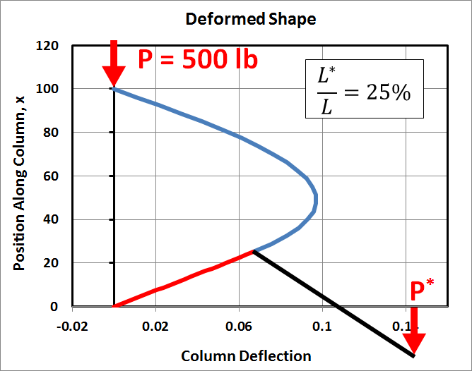
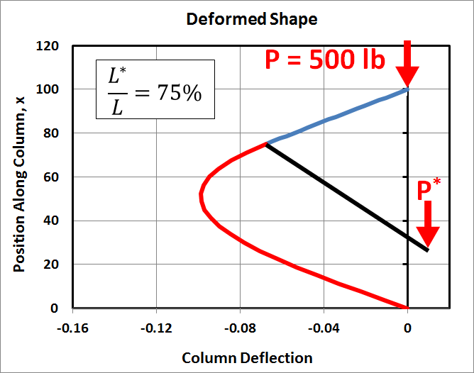
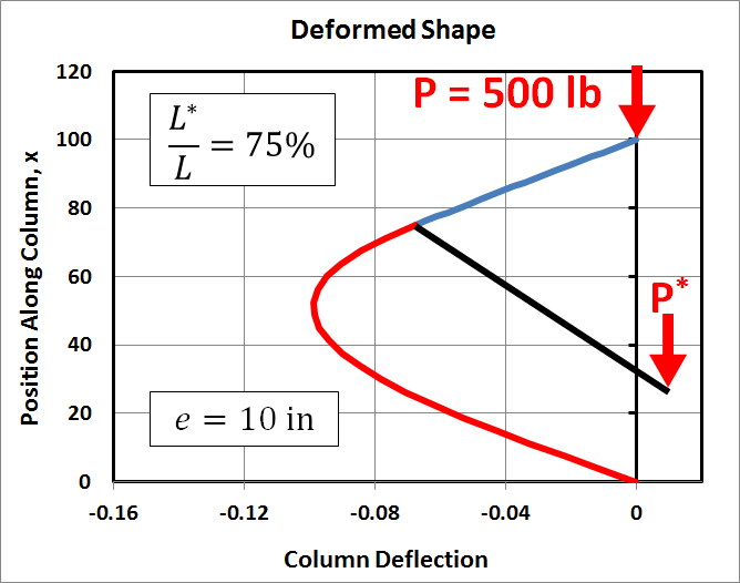
We will first start with a load of \(P = 500\,\text{lb}\), which is small compared to the critical load, and the eccentric load is \(P^* = 10\,\text{lb}\) at \(e = 10\,\text{in}\).
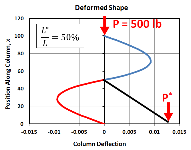
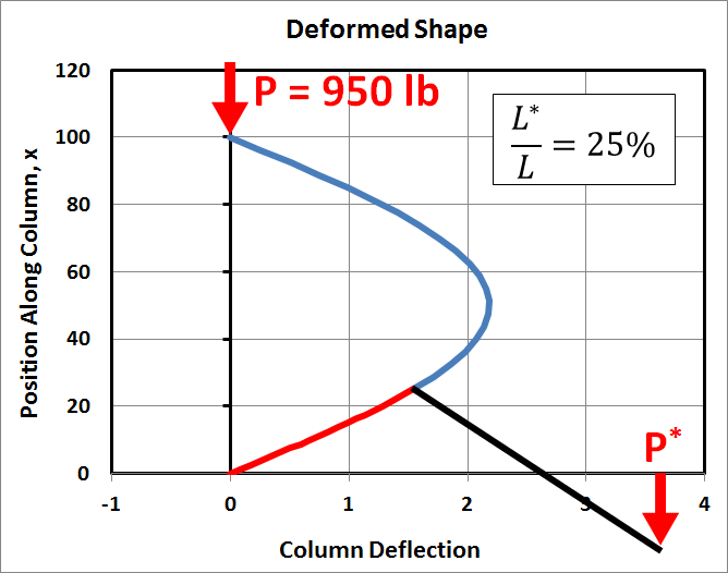
Finally the eccentric load will be located at 75%, 50%, and 25% of the beam's length. The graphs below show the resulting column deflections. Several items are worth noting:
- The column deflections are antisymmetric. For example, in the 75% case, it moves about 0.1" to the left, while in the 25% case, it moves an equal amount to the right.
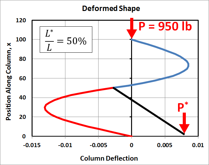
- In the 50% case, the deflections are antisymmetric above and below the eccentric load.
- The deflections in the 50% case are substantially less than in the 25% or 75% cases.
- In every case, the deflections are such that the eccentric load, \(P^*\), moves downward.
- The black cantilevered portion is not drawn to scale.
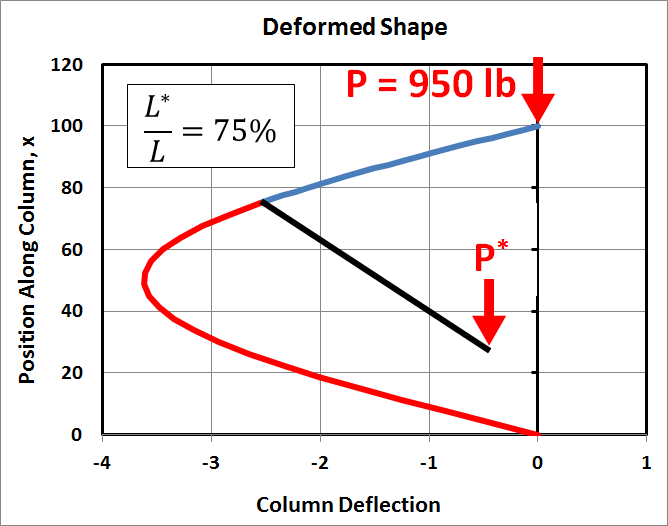
This time, the only thing that has changed is that \(P\) has increased from 500 lb to 950 lb, or 98% of \(P_{cr}\). As can be seen the resulting deflections are significantly greater than before, at least for \(L^*\) at 25% and 75% of \(L\). Also, they are no longer antisymmetric. This is because the eccentric load, \(P^*\), itself is not symmetric. It is cantilevered off one side of the column. Furthermore, the compressive load in the column above it is \(P\), while the compressive load is \(P+P^*\) below it.
In the first case, when \(P = 500\,\text{lb}\), the addition of \(10\,\text{lb}\) was still small compared to the critical load of \(972\,\text{lb}\). However, in this case, when \(P = 950\,\text{lb}\), the addition of ten more pounds represents a significant step closer to the critical load.
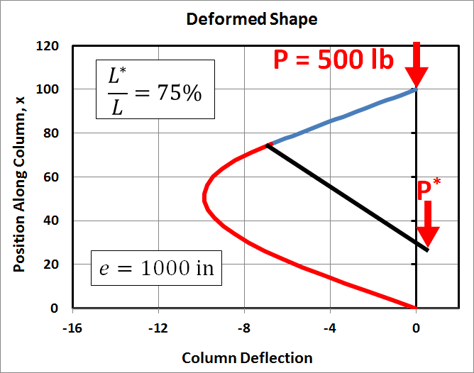
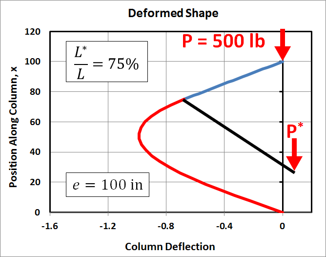
This time, we hold everything constant except the eccentricity, \(e\). The following three cases are similar to the first, with \(P = 500\,\text{lb}\) and with \(P^*\) located at 75% of \(L\). But the eccentricity takes on values of 10 in, 100 in, and 1000 in.
Note that the displacements are directly proportional to the eccentricity. This should not be a surprise, in fact, because it is also true in classical eccentric buckling analyses. It is also apparent in the solution to the multiload buckling equations here because the equations for the constants of integration are directly proportional to \(e\).
Stresses
In order to calculate the stresses, it is first necessary to compute the internal bending moments throughout the column. The moments can be calculated by either of two approaches. The first is to take the second derivative of the deflection equations and relate them to the bending moment using \(E \, I \, y'' = M\).The alternative is to insert the deflection equations into
\[ \begin{eqnarray} \text{Top:} & \qquad M^{top} & = & {P^* e \over L} (L - x) - P \, y^{top} \\ \\ \text{Bottom:} & \qquad M^{bot} & = & - \, {P^* e \over L} \, x - (P + P^*) \, y^{bot} \end{eqnarray} \]
Both approaches lead to
\[ \begin{eqnarray} \text{Top:} & \qquad M^{top} = & - P \, T \left[ \sin \left( \sqrt{ P \over E \, I} \, x \right) - \tan \left( \sqrt{ P \over E \, I} \, L \right) \cos \left( \sqrt{ P \over E \, I} \, x \right) \right] \\ \\ \\ \text{Bottom:} & \qquad M^{bot} = & - (P + P^*) \, B \, \sin \left( \sqrt{ P + P^* \over E \, I} \, x \right) \end{eqnarray} \]
The bending moment expressions are inserted into the following equation to obtain the stresses
\[ \sigma_{comp} = \left| \, F \over A \, \right| + \left| M c \over I \right| \]
where \(c\) is the maximum \(\text{y}\)-value measured from the neutral axis, and \(F\) is equal to \(P\) above \(L^*\) and \(P + P^*\) below \(L^*\). Absolute values are taken to obtain the maximum compressive stress as a positive result for graphs. Positive values are used for \(P\) and \(P^*\). Note that technically, this stress is negative because it is compressive. The result is
\[ \begin{eqnarray} \text{Top:} & \qquad \sigma^{top} = & {P \over A } + {P \, |T| \, c \over I} \left[ \sin \left( \sqrt{ P \over E \, I} \, x \right) - \tan \left( \sqrt{ P \over E \, I} \, L \right) \cos \left( \sqrt{ P \over E \, I} \, x \right) \right] \\ \\ \\ \text{Bottom:} & \qquad \sigma^{bot} = & {P + P^* \over A \,} + { (P + P^*) \, |B| \, c \over I } \sin \left( \sqrt{ P + P^* \over E \, I} \, x \right) \end{eqnarray} \]
Normalizing the equations by \(P_{cr}\) again gives
\[ \begin{eqnarray} \text{Top:} & \qquad \sigma^{top} = & {P \over A} + {P \, |T| \, c \over I} \left[ \sin \left( \pi \sqrt{P \over P_{cr}} \, {x \over L} \right) - \tan \left( \pi \sqrt{ P \over P_{cr}} \, \right) \cos \left( \pi \sqrt{ P \over P_{cr}} {x \over L} \right) \right] \\ \\ \\ \text{Bottom:} & \qquad \sigma^{bot} = & {P + P^* \over A \,} + { (P + P^*) \, |B| \, c \over I } \sin \left(\pi \sqrt{P + P^* \over P_{cr}} \, {x \over L} \right) \end{eqnarray} \]
And the two BC equations are repeated here to keep the complete set of four equations together.
\[ \begin{eqnarray} T \left[ \sin \left( \pi \sqrt{ P \over P_{cr}} \, {L^* \over L\;} \right) - \tan \left( \pi \sqrt{ P \over P_{cr}} \, \right) \cos \left( \pi \sqrt{ P \over P_{cr}} \, {L^* \over L\;} \right) \right] - B \, \sin \left( \pi \sqrt{ P + P^* \over P_{cr}} \, {L^* \over L\;} \right) = - \left[ { P^* \over P \, } \left( 1 - {L^* \over L} \right) + { P^* \over P + P^* } \left( L^* \over L \right) \right] e \\ \\ \\ T \, \pi \, \sqrt{ P \over P_{cr}} \left[ \cos \left( \pi \sqrt{ P \over P_{cr}} \, {L^* \over L\;} \right) + \tan \left( \pi \sqrt{ P \over P_{cr}} \, \right) \sin \left( \pi \sqrt{ P \over P_{cr}} \, {L^* \over L\;} \right) \right] - B \, \pi \, \sqrt{ P + P^* \over P_{cr}} \cos \left( \pi \sqrt{ P + P^* \over P_{cr}} \, {L^* \over L\;} \right) = \left( P^* \over P\, \right) \left( P^* \over P + P^* \right) e \end{eqnarray} \]
Dimensionless Terms
The stress equations are easily arranged to obtain dimensionless terms as follows.\[ \begin{eqnarray} \text{Top:} & \qquad \sigma^{top} = & {P \over A} \left\{ 1 + {A \, |T| \, c \over I} \left[ \sin \left( \pi \sqrt{P \over P_{cr}} \, {x \over L} \right) - \tan \left( \pi \sqrt{ P \over P_{cr}} \, \right) \cos \left( \pi \sqrt{ P \over P_{cr}} {x \over L} \right) \right] \right\} \\ \\ \\ \text{Bottom:} & \qquad \sigma^{bot} = & {P + P^* \over A \,} \left\{ 1 + { A \, |B| \, c \over I } \sin \left(\pi \sqrt{P + P^* \over P_{cr}} \, {x \over L} \right) \right\} \end{eqnarray} \]
Note that these equations are very similar to those of eccentric buckling theory. The eccentric buckling results contain the term, \(A e c / I\), whereas this solution contains the terms, \(A |T| c / I\) and \(A |B| c / I\). But recall that \(T\) and \(B\) are both proportional to \(e\), so the similarities are even stronger than first appearances suggest.
This arrangement also puts the equations in forms that isolate the compression and bending contributions as follows.
\[ \sigma^{top} = {P \over A} \, \Big[ 1 + \text{Bending Terms} \Big] \qquad \quad \text{and} \qquad \quad \sigma^{bot} = {P+P^* \over A} \, \Big[ 1 + \text{Bending Terms} \Big] \]
So the max compressive stress in the column at any point starts at \(P / A\), or \((P + P^*) / A\), and is then amplified by the bending moment(s) due to \(P\) and \(P^*\). Interestingly, there is no bending in the column at its two ends, \(x = 0\) and \(x = L\), so \(\sigma = P / A\) and \(\sigma = (P + P^*) / A\) at these two extremes. This will be clear in the graphs below.
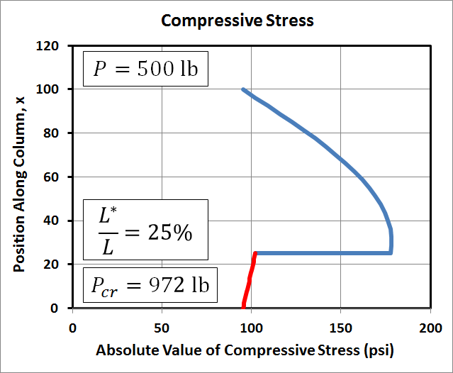
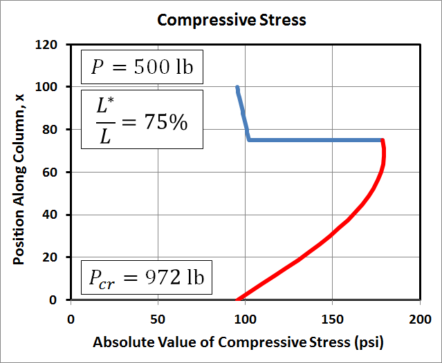
Column Stress Examples
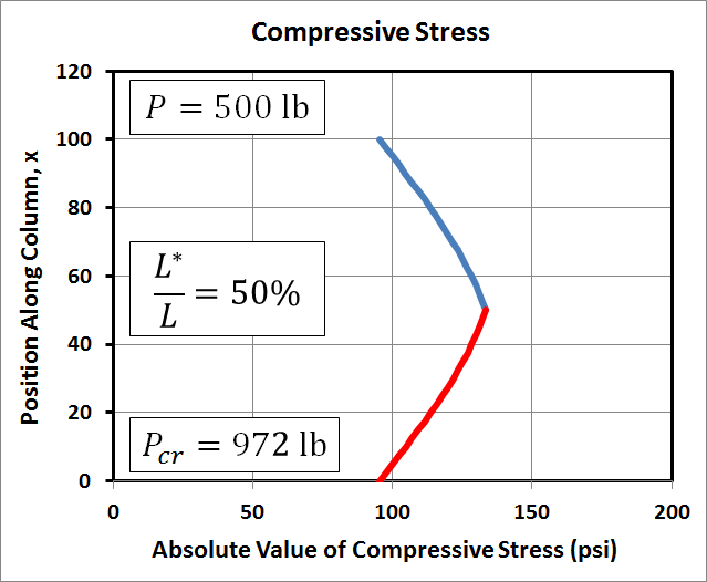
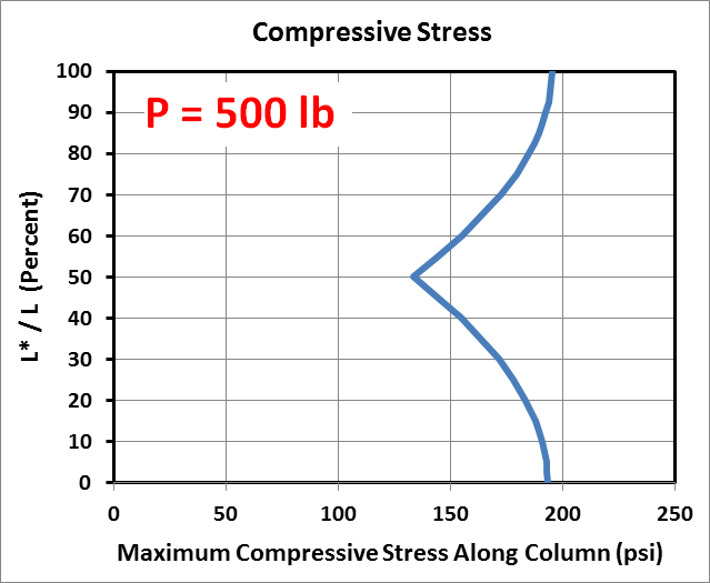
The graphs here of maximum compressive stress in the column correspond to the same conditions (length, load, area, etc) as those in the deflection example above. For completeness, the cross-section is 1.5"x3.5", the modulus is 1E+6 psi, the length is 100", the eccentricity is 10", and \(P^*\) = 10 lb. And all of this leads to \(P_{cr}\) = 972 lb.The first row of graphs correspond to \(P\) = 500 lb. Like the deflections, the stress plots are symmetric, or antisymmetric depending on your point of view. The stress level at the top and bottom of the column is \(P / A\) (and \((P+P^*)/A\)) where the bending moment is zero. It increases due to bending in between. Interestingly, the maximum stress when \(L^*/L = 50%\) is lower than when \(L^*/L\) is 25% or 75%.
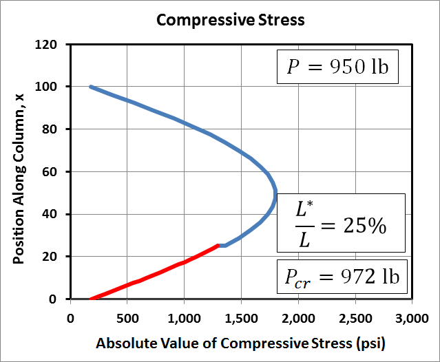
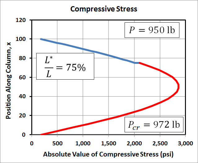
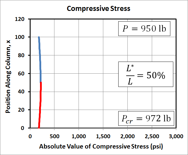
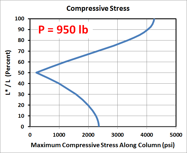
As with the deflection example, the only thing that has changed this time is that \(P\) has increased from 500 lb to 950 lb, or 98% of \(P_{cr}\). As can be seen the resulting stresses are significantly greater now than before, at least for \(L^*\) at 25% and 75% of \(L\). Also, they are no longer symmetric. The 75% case has higher stress than the 25% case.
Finally, note that although \(P\) has not quite doubled in value, the resulting stresses have increased by an order of magnitude. This is because the compressive load of 950 lb is very close to \(P_{cr}\). The stresses will continue to grow exponentially as \(P\) approaches \(P_{cr}\).
There is no need to plot stresses versus eccentricity as was done in the above example. This is because the stresses are directly related to the deflections, and therefore directly proportional to the eccentricity as were the deflections.
More Column Stress Examples
The dependence of stress on \(L^*/L\) in the above example is very interesting. The graphs below explore this dependence in more depth, plotting the maximum compressive stress at any point in the column as a function of \(L^*/L\). They show that the minimum stress occurs when the cantilevered load is at precisely 50% of the column's height.When the load, \(P\), is small compared to \(P_{cr}\), then the highest stress occurs when \(P^*\) is at either 0% or 100% of the column's height. However, once \(P\) approaches \(P_{cr}\), then it becomes clear that placing \(P^*\) near the top of the column produces significantly higher stresses than when \(P^*\) is near the bottom, even though it is only 10 lb in this example.
And once again, keep in mind that although \(P\) increased by only 90%, the stresses in the column increase by an order of magnitude because in the second case, \(P\) is close to \(P_{cr}\).
|
|
Buckling Criteria
This section establishes buckling criteria for the multiload column case in terms of \(P\) and \(P^*\). The process is involved, but the result is a straight-forward reference graph that is easily interpreted. It starts from a point that will initially seem surprising, the boundary condition equations for \(T\) and \(B\).Writing the two equations in matrix form gives
\[ \left[ \matrix{ \sin \left( \pi \sqrt{ P \over P_{cr}} \, {L^* \over L\;} \right) - \tan \left( \pi \sqrt{ P \over P_{cr}} \, \right) \cos \left( \pi \sqrt{ P \over P_{cr}} \, {L^* \over L\;} \right) & - \sin \left( \pi \sqrt{ P + P^* \over P_{cr}} \, {L^* \over L\;} \right) \\ \\ \pi \, \sqrt{ P \over P_{cr}} \left[ \cos \left( \pi \sqrt{ P \over P_{cr}} \, {L^* \over L\;} \right) + \tan \left( \pi \sqrt{ P \over P_{cr}} \, \right) \sin \left( \pi \sqrt{ P \over P_{cr}} \, {L^* \over L\;} \right) \right] & - \pi \, \sqrt{ P + P^* \over P_{cr}} \cos \left( \pi \sqrt{ P + P^* \over P_{cr}} \, {L^* \over L\;} \right) } \right] \left\{ \matrix{ T \\ \\ \\ B } \right\} = \left\{ \matrix{ - \left[ { P^* \over P \, } \left( 1 - {L^* \over L} \right) + { P^* \over P + P^* } \left( L^* \over L \right) \right] e \\ \\ \left( P^* \over P\, \right) \left( P^* \over P + P^* \right) e } \right\} \]
The key is to recognize that under certain conditions, the determinant of the above matrix equation can go to zero. This drives the corresponding values of \(T\) and \(B\) to infinity in order to satisfy the equation. And since both deflections and stresses depend directly on \(T\) and \(B\), they go to infinity as well. This is the buckling criterion.
So buckling occurs whenever the determinant of the matrix of boundary conditions equals zero. In other words...
\[ \begin{eqnarray} - \pi \, \sqrt{ P + P^* \over P_{cr}} \left[ \sin \left( \pi \sqrt{ P \over P_{cr}} \, {L^* \over L\;} \right) - \tan \left( \pi \sqrt{ P \over P_{cr}} \, \right) \cos \left( \pi \sqrt{ P \over P_{cr}} \, {L^* \over L\;} \right) \right] \cos \left( \pi \sqrt{ P + P^* \over P_{cr}} \, {L^* \over L\;} \right) + \quad \qquad \\ \\ \qquad \quad \pi \, \sqrt{ P \over P_{cr}} \left[ \cos \left( \pi \sqrt{ P \over P_{cr}} \, {L^* \over L\;} \right) + \tan \left( \pi \sqrt{ P \over P_{cr}} \, \right) \sin \left( \pi \sqrt{ P \over P_{cr}} \, {L^* \over L\;} \right) \right] \sin \left( \pi \sqrt{ P + P^* \over P_{cr}} \, {L^* \over L\;} \right) = 0 \end{eqnarray} \]
which is clearly, a mess. But fortunately, it is possible to greatly simplify the equation. First, cancel the leading \(\pi\) from each term. Second, combine the two leading \(\sqrt{\;\;}\) terms into a single \(\sqrt{ P \over P + P^*}\) term. Finally, divide through by both \( \cos \left( \pi \sqrt{ P \over P_{cr}} \, {L^* \over L\;} \right) \) and \( \cos \left( \pi \sqrt{ P + P^* \over P_{cr}} \, {L^* \over L\;} \right) \). This will cancel several of the \(\cos()\) terms and convert several more \(\sin()\) terms into \(\tan()\) functions. All this simplifies the equation to
\[ - \left[ \tan \left( \pi \sqrt{ P \over P_{cr}} \, {L^* \over L\;} \right) - \tan \left( \pi \sqrt{ P \over P_{cr}} \, \right) \right] + \sqrt{ P \over P + P^*} \left[ 1 + \tan \left( \pi \sqrt{ P \over P_{cr}} \, \right) \tan \left( \pi \sqrt{ P \over P_{cr}} \, {L^* \over L\;} \right) \right] \tan \left( \pi \sqrt{ P + P^* \over P_{cr}} \, {L^* \over L\;} \right) = 0 \]
Next, rearrange the terms as follows.
\[ - \; { \tan \left( \pi \sqrt{ P \over P_{cr}} \, \right) - \tan \left( \pi \sqrt{ P \over P_{cr}} \, {L^* \over L\;} \right) \over 1 + \tan \left( \pi \sqrt{ P \over P_{cr}} \, \right) \tan \left( \pi \sqrt{ P \over P_{cr}} \, {L^* \over L\;} \right) } \; = \; \sqrt{ P \over P + P^*} \; \tan \left( \pi \sqrt{ P + P^* \over P_{cr}} \, {L^* \over L\;} \right) \]
And recognize that the left hand side of the equation matches the following trig identity.
\[ \tan(\alpha - \beta) = {\tan(\alpha) - \tan(\beta) \over 1 + \tan(\alpha) \, \tan(\beta) } \]
So it can be further simplified to
\[ - \; \tan \left[ \pi \sqrt{ P \over P_{cr}} \left( 1 - {L^* \over L\;} \right) \right] \; = \; \sqrt{ P \over P + P^*} \; \tan \left( \pi \sqrt{ P + P^* \over P_{cr}} \, {L^* \over L\;} \right) \]
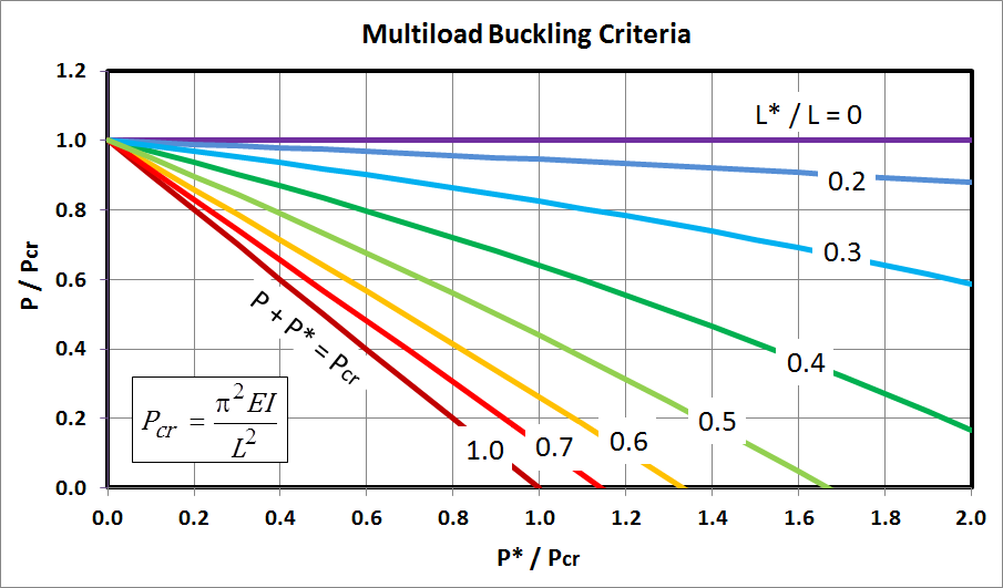
And that is about as good as it gets. It's much better than the start, but still requires numerical solution. However, the good news is that the solutions can be computed once, and then plotted. This will be done. But even before that, there is one more thing to do. It is to group parameters together into convenient dimensionless terms. They are \(P \over P_{cr}\), \(P^* \over P_{cr}\), and \(L* \over L\). Doing so gives
\[ - \; \tan \left[ \pi \sqrt{ P \over P_{cr}} \left( 1 - {L^* \over L\;} \right) \right] \; = \; \sqrt{ P/P_{cr} \over P/P_{cr} + P^*/P_{cr}} \; \tan \left( \pi \, \sqrt{ {P \over P_{cr}} + {P^* \over P_{cr}}} \; {L^* \over L\;} \right) \]
It is possible to think of the equation as expressing \(P/P_{cr}\) as a function of \(P^*/P_{cr}\) for any given value of \(L^*/L\). This is in fact done for several values of \(L^*/L\) in the graph below.
There are many important aspects of the buckling criterion to review.
- It shares important properties with classical eccentric buckling theory.
- The critical buckling load, \(P_{cr}\), becomes a bit of an academic
value because all eccentrically loaded columns will in fact fail at loads
less than \(P_{cr}\) because the stresses in the columns will exceed
the material's yield strength first. (This is not the case in classical
Euler buckling theory because it does not have an eccentric load.)
- There is no dependence at all of the critical buckling load on
eccentricity, \(e\). It is not present in the buckling criterion equation.
Nevertheless, eccentricity does play a very important role in reality
because column deflections and stress are proportional to it.
And as was just stated, eccentrically loaded columns actually fail
due to stresses exceeding yield strengths.
- The critical buckling load, \(P_{cr}\), becomes a bit of an academic
value because all eccentrically loaded columns will in fact fail at loads
less than \(P_{cr}\) because the stresses in the columns will exceed
the material's yield strength first. (This is not the case in classical
Euler buckling theory because it does not have an eccentric load.)
- However, it does have an important difference from classical eccentric
buckling theory.
- Whereas classical eccentrically loaded columns buckle (not yield,
but buckle) at the fixed load, \(P_{cr}\), independent of other parameters
such as eccentricity, that is not the case here with the multiloaded column.
Here, the column buckles at loads different from, and in fact less than, \(P_{cr}\).
This makes the \(P_{cr}\) parameter even more of an academic value that should
not be confused with the load(s) at which a multiloaded column actually collapses.
- Finally, there are several important properties to address concerning the above chart itself.
- In general, the greater the value of \(L^* / L\), the lower the buckling
threshold of the column.
- When \(L^*/L = 0\), there is no influence of \(P^*\)
on buckling at all. The column buckles at \(P = P_{cr}\) regardless of the
values of \(P^*\) and \(e\). But don't forget about yielding - - \(P^*\) and
\(e\) will still significantly influence the stresses in the column.
- At the other extreme, when \(L^*/L = 1\), the buckling criterion simplifies
to \(P + P^* = P_{cr}\). In other words, \(P\) and \(P^*\) are of equal
importance, and it is simply their sum that is the critical value.
- In between, an increase in \(P^*\) results in a decrease in allowable
\(P\), but by an amount less than the original increase in \(P^*\).
- Note that \(P^*\) can significantly exceed \(P_{cr}\) without triggering
buckling, but by smaller and smaller amounts as \(L^* / L\) increases.
- There is little difference in buckling behavior once \(L^* / L\) exceeds 70%. In effect, once 70% or more of the length of the column supports \(P + P^*\), then it behaves effectively as if the entire length does.
- In general, the greater the value of \(L^* / L\), the lower the buckling
threshold of the column.
Buckling Example
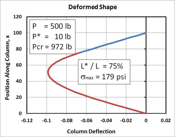
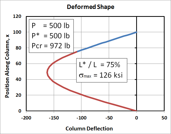
Here we continue the example of the 100" long 2"x4" (with \(e\) = 10") and get to the subject of just when will this column collapse.The left graph below is a repeat of the above example(s) in which \(P\) = 500 lb. The deflections are small and the chart also states that the maximum stress in the column is (only) 179 psi. The graph is provided for reference.
In the right graph, the eccentric load, \(P^*\), has increased to 500 lb. The resulting predicted deflections and stresses are now impossibly large. Nevertheless, the column still has not buckled, even though the sum of \(P\) and \(P^*\) is greater than \(P_{cr}\). (Note that although it has not buckled in the theoretical sense, it may have already failed in reality due to the very high stress. This is why stress levels must always be checked.)
|
|
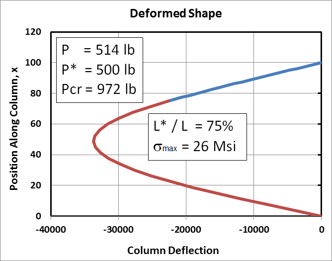
The eccentric load is held constant at 500 lb in the two graphs below. The only difference between them and the above graph is the value of \(P\). In the left graph, \(P\) has increased to 514 lb. This is the critical load, as evidenced by the preposterously high deflections and stresses.
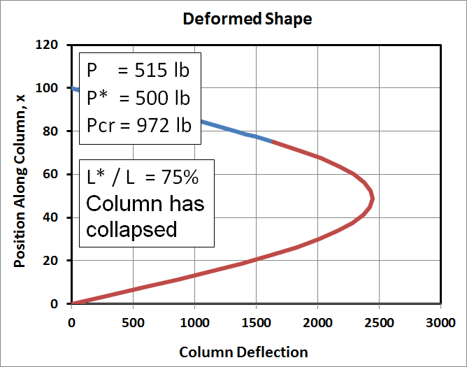
In the right graph, \(P\) has increased by 1 lb to 515 lb. This has caused the column to buckle, as evidenced by the sudden change in sign of the deflections. All values in this graph, both deflections and stresses, are in fact meaningless.
|
|
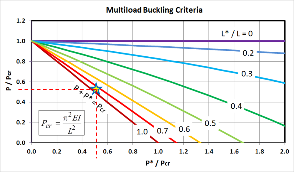
Plotting these results on the buckling graph shows that all of the analyses are in fact consistent. The key points on the graph are
\[ {P \over P_{cr}} = {514 \text{ lb} \over 972 \text{ lb}} = 0.53 \qquad \qquad {P^* \over P_{cr}} = {500 \text{ lb} \over 972 \text{ lb}} = 0.51 \qquad \qquad {L^* \over L} = { 75 \text{ in} \over 100 \text{ in}} = 0.75 \]
Summary
So, to summarize... for the situation shown at the right, \(P_{cr}\) is given by\[ P_{cr} = {\pi^2 E \, I \over L^2} \]
but keep in mind that this is only an academic quantity here. The column will actually buckle at lower loads whenever \(P^*\) and \(L^*\) are greater than zero.
The column deflections are given by the following equations (where top and bot refer to the portions of the column above and below the cantilevered load, \(P^*\)).
\[ \begin{eqnarray} \text{Top:} & \qquad y^{top} = & T \left[ \sin \left( \pi \sqrt{P \over P_{cr}} \, {x \over L} \right) - \tan \left( \pi \sqrt{ P \over P_{cr}} \, \right) \cos \left( \pi \sqrt{ P \over P_{cr}} {x \over L} \right) \right] + { P^* \over P \, } \left( 1 - {x \over L} \right) e \\ \\ \\ \text{Bottom:} & \qquad y^{bot} = & B \, \sin \left(\pi \sqrt{P + P^* \over P_{cr}} \, {x \over L} \right) - { P^* \over P + P^* } \left( x \over L \right) e \end{eqnarray} \]
And the resulting stresses are
\[ \begin{eqnarray} \text{Top:} & \qquad \sigma^{top} = & {P \over A} \left\{ 1 + {A \, |T| \, c \over I} \left[ \sin \left( \pi \sqrt{P \over P_{cr}} \, {x \over L} \right) - \tan \left( \pi \sqrt{ P \over P_{cr}} \, \right) \cos \left( \pi \sqrt{ P \over P_{cr}} {x \over L} \right) \right] \right\} \\ \\ \\ \text{Bottom:} & \qquad \sigma^{bot} = & {P + P^* \over A \,} \left\{ 1 + { A \, |B| \, c \over I } \sin \left(\pi \sqrt{P + P^* \over P_{cr}} \, {x \over L} \right) \right\} \end{eqnarray} \]
And the two BC equations used to determine \(T\) and \(B\) are
\[ \begin{eqnarray} T \left[ \sin \left( \pi \sqrt{ P \over P_{cr}} \, {L^* \over L\;} \right) - \tan \left( \pi \sqrt{ P \over P_{cr}} \, \right) \cos \left( \pi \sqrt{ P \over P_{cr}} \, {L^* \over L\;} \right) \right] - B \, \sin \left( \pi \sqrt{ P + P^* \over P_{cr}} \, {L^* \over L\;} \right) = - \left[ { P^* \over P \, } \left( 1 - {L^* \over L} \right) + { P^* \over P + P^* } \left( L^* \over L \right) \right] e \\ \\ \\ T \, \pi \, \sqrt{ P \over P_{cr}} \left[ \cos \left( \pi \sqrt{ P \over P_{cr}} \, {L^* \over L\;} \right) + \tan \left( \pi \sqrt{ P \over P_{cr}} \, \right) \sin \left( \pi \sqrt{ P \over P_{cr}} \, {L^* \over L\;} \right) \right] - B \, \pi \, \sqrt{ P + P^* \over P_{cr}} \cos \left( \pi \sqrt{ P + P^* \over P_{cr}} \, {L^* \over L\;} \right) = \left( P^* \over P\, \right) \left( P^* \over P + P^* \right) e \end{eqnarray} \]
The buckling criterion for the multiloaded column is governed by
\[ - \; \tan \left[ \pi \sqrt{ P \over P_{cr}} \left( 1 - {L^* \over L\;} \right) \right] \; = \; \sqrt{ P \over P + P^*} \; \tan \left( \pi \sqrt{ P + P^* \over P_{cr}} \, {L^* \over L\;} \right) \]
It is independent of \(e\) and must be solved numerically. This is done and plotted in the graph below.
Some general notes about the results are...
- The maximum load the beam can support is \(P_{cr}\), as expected.
However, it can also buckle at lower loads when \(P^*\) and \(L^*\) are large.
It will in fact fail at even lower loads because the stresses in it will exceed the yield strength
of the material. So both criteria must be checked. (High stresses result primarily
from bending caused by the eccentric load, \(P^*\).)
- One can obtain computed deflections and stresses at loads
exceeding the buckling strength of the column, but they are meaningless because
the column will have already collapsed. The best indication of
collapse, besides checking the above graph, is that the computed deflections have the wrong
sign. See examples above to learn how to recognize this situation.
- Placing \(P^*\) at half the column height (\(L^* / L = 0.5\)) produces the
lowest stresses. But the stress solution is very sensitive to this height
and increases sharply as \(P^*\) is raised or lowered from this midpoint.
- Placing \(P^*\) in the upper half of the column produces higher stresses
than if it were in the lower half. This can be thought of in terms of the
amount of column length supporting \(P\) versus \(P+P^*\).
- Placing \(P^*\) at the full height of the column (\(L^* = L\)) produces the highest stresses.
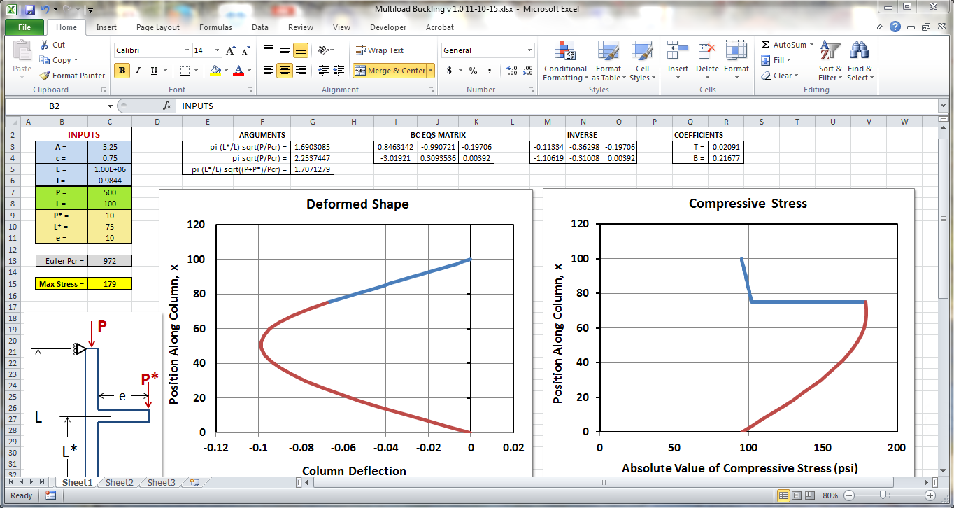
This spreadsheet computes the column deflections and stresses. You are welcome to use it at your own risk. I make no claims of its accuracy and am not responsible for the results.
Remember, it is entirely possible to input values that exceed buckling conditions and still get what may appear to be reasonable results, but they are not. The predictions are meaningless when the column has buckled. A common symptom of this is that the predicted column deflections have the wrong sign and result in the offset force, \(P^*\), moving up instead of down on the deformed column. Refer to the above examples involving column deflections for additional details.