Column Buckling

Introduction

Column buckling is a curious and unique subject. It is perhaps the only area of structural mechanics in which failure is not related to the strength of the material. A column buckling analysis consists of determining the maximum load a column can support before it collapses. But for long columns, the collapse has nothing to do with material yield. It is instead governed by the column's stiffness, both material and geometric.

This page will derive the standard equations of column buckling using two approaches. It will first cover the usual development of the equations, i.e., Euler Buckling Theory. This is the derivation found in text books and presented in engineering courses. But I have never liked it. Not because it is incorrect (it is correct), but because I don't think it satisfactorily presents the physical mechanisms governing the buckling process. That is why a second derivation of the buckling equations will also be presented.

Curiously, objects are referred to as columns when they are loaded axially in compression, as is the case here, but they are referred to as beams when they are loaded transversely. Nevertheless, beam bending theory is central to column buckling analyses, so it is recommended that the reader review this beam bending page.

Euler Buckling Theory

Euler Buckling Theory is the classical theory presented in textbooks and classrooms. It begins simply by noting that the internal bending moment in a loaded and deformed column is \(-P \, y\) where \(P\) is the compressive load and \(y\) is the column deflection. So insert \(-P \, y\) in for \(M\) in the beam bending equation, \( E \, I \, y'' = M \).

\[ E \, I \, y'' = M = -P \, y \]
This produces the following differential equation

\[ E \, I \, y'' + P \, y = 0 \]
which has the solution

\[ y = A \sin \left( \sqrt{{P \over E \, I}} \; x \right) + B \cos \left( \sqrt{{P \over E \, I}} \; x \right) \]
where \(A\) and \(B\) are constants determined from the boundary conditions.

The boundary conditions are \(y = 0\) at \(x = 0\) and \(x = L\).

The first boundary condition, \(y = 0\) at \(x = 0\), leads to the conclusion that \(B = 0\). And this leaves

\[ y = A \sin \left( \sqrt{{P \over E \, I}} \; x \right) \]
So far, so good. But it's at this point that the classical derivation tends to leave physical intuition behind and become overtly mathematical...

Things become very interesting with the 2nd boundary condition because, as we will see, it does not lead to determination of the unknown constant, \(A\). To see this, insert the second boundary condition as follows.

\[ y(L) = 0 = A \sin \left( \sqrt{{P \over E \, I}} \; L \right) \]
There are basically two possibilities here. In the first case, \(A = 0\), but this is boring because it leads to the result that all displacements are zero. This is just the nonbuckled solution. Before the column buckles, its lateral displacements are simply zero.

The second case is the interesting one, and the one directly related to column buckling. The second method of satisfying the boundary condition is to note that \(\sin(\pi) = 0\). Therefore the way to satisfy the boundary condition is to require that the argument in the equation, \(\left( \sqrt{{P \over E \, I}} \; L \right)\) must equal \(\pi\). Doing so gives

\[ \sqrt{{P \over E \, I}} \; L = \pi \]
and solving for \(P\) gives

\[ P_{cr} = { \pi^2 \, E \, I \over L^2 } \]
This is the classical Euler buckling theory result. It gives the critical value of load \(P\), called \(P_{cr}\), above which, the column will buckle.

This result is perfectly legit. However, as should be evident by now, it is very mathematical in nature, and provides little physical insight as a result. The up-coming derivation below will present an alternative method of arriving at the same equation that I believe provides a much more direct physical connection to the buckling process than the above derivation did.

Buckling vs Yielding

As stated at the outset, classical buckling analysis is independent of a material's yield strength. This is evident in the above derivation because at no time was stress or strain discussed or compared to a material's strength.

But in fact, yielding considerations should never be totally ignored. Once one obtains an estimate of \(P_{cr}\) from the above equation, one should always divide it by the column's cross-sectional area, \(A\), to obtain a stress

\[ \sigma_x = { P_{cr} \over A } \]
and compare this value to the material's yield strength to determine if yielding will occur before buckling. This is critical for short columns since they have inherently high \(P_{cr}\) values because \(L^2\) is in the denominator of the buckling equation.

End Constraints in Buckling

Though not the focus of this page, it is important to recognize that end constraints are critical to buckling analyses because they alter the value of \(P_{cr}\). For example, consider that the critical buckling load of the column shown here is given by

\[ P_{cr} = { \pi^2 \, E \, I \over 4 \, L^2 } \]
Note that this value is 1/4 that given in the earlier equation for \(P_{cr}\). But it is easy to see why. The sketch shows that the buckling condition here is exactly equivalent to the buckling of a column of twice the length and having the same boundary conditions as in the above derivation. And this leads to

\[ P_{cr} = { \pi^2 \, E \, I \over ( 2 \, L)^2 } = { \pi^2 \, E \, I \over 4 \, L^2 } \]

Physically-Based Buckling Derivation

This section will present an alternative method of determining critical buckling loads that I believe is more physically intuitive than classical Euler buckling theory. Its key feature is the comparison of the internal bending moment arising from the internal stress distribution to the external bending moment resulting from the load applied to the column. (The previous sentence is critical.)

This approach picks up approximately where it was noted earlier that the classical Euler approach becomes overtly mathematical. The first step is to assume a deformed shape. We know that \(y = 0\) at both ends of the column, and that the shape follows a \(\sin()\) function based on the above differential equation. So the most logical choice is

\[ y(x) = \delta_{max} \sin ( {\pi x \over L} ) \]
where \(\delta_{max}\) is the lateral displacement at the midpoint of the column. Its value is unknown, but it is known to be greater at the midpoint than at any other point on the column, hence the \(max\) subscript. The choice of \(\pi x / L\) as the argument of the \(\sin()\) function ensures that the displacements are zero at \(x = 0\) and \(x = L\). (We will talk about other assumed shapes shortly.)

If you are wondering about the \(\sqrt{P/EI}\) term in the \(\sin()\) function from the earlier Euler solution, don't. It arose from the solution of the differential equation, but we are pretending to know nothing about the details of that solution here (exception alert!). We only need a function that can resemble a bowed column with zero displacements at its ends. Using \(\sin ( {\pi x \over L} )\) accomplishes this.

The "exception alert" is present above because we are in fact taking advantage of one piece of knowledge about the earlier analysis. It is that trig functions are the solutions of the differential equation. Therefore, sines and cosines should be used whenever possible to describe the deformed shapes because they will lead to the most accurate estimates of \(P_{cr}\).

Recall from beam bending theory that the bending moment, \(M\), is related to the deflection of the column by

\[ M = E \, I \, y'' \]
Though not critical, it is helpful to remember that this relationship came from calculating the moment in the cross-section due to the stress distribution. The relationship shows that we need the second derivative of the assumed displacement function.

\[ \begin{eqnarray} M \; = \; E \, I \, y'' \; & = & \; E \, I \, {d^2 \over dx^2 } \left\{ \delta_{max} \sin ( {\pi x \over L} ) \right\} \\ \\ \\ & = & \; - {\pi^2 \, E \, I \, \delta_{max} \over L^2 } \sin ( {\pi x \over L} ) \\ \\ \\ & = & \; - {\pi^2 \, E \, I \, y(x) \over L^2 } \end{eqnarray} \]
This is the internal bending moment in the column due to the stress distribution within it, which is in turn due to the fact that the column is bent.

Here comes an important thought... This bending moment can be thought of as the column's internal resistance to bending, or the strength with which it tries to straighten back out.

The simple next-step is to equate this internal resistive bending moment to that resulting from the external load. That amount is simply \(M = -P \, y(x)\). Equating the two gives

\[ M \; = \; -P \, y(x) \; = \; - {\pi^2 \, E \, I \, y(x) \over L^2 } \]
It is not hard to see at this point that this approach is leading to the same expression for \(P_{cr}\) as the classical Euler buckling theory did. But along the way, it has provided much more insight into the physical process of buckling than the former theory. Namely...

We have arrived at this relationship by equating the internal bending moment (due to the internal stresses arising from the column's bending) to the external bending moment resulting from the external load, \(P\). It should be clear that buckling occurs when \(P\) is large enough to satisfy the equation. Any value less, and \(P \, y(x)\) will be less than the "resisting bending moment."
The fact that \(y(x)\) appears on both sides of the equation, and will therefore be cancelled out, means that when buckling does occur, it does so simultaneously throughout the length of the column. (A fascinating result that is not evident in the Euler theory.)

Anyway, cancelling out \(y(x)\) from both sides of the equation gives

\[ P_{cr} = { \pi^2 \, E \, I \over L^2 } \]
again, but with much more physical insight this time.

Fixed End Example

This time, assume a deformed shape of

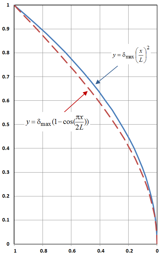
\[ y = \delta_{max} ( 1 - \cos ( { \pi x \over 2 L }) ) \]
Calculate the bending moment due to this.

\[ M \; = \; E \, I \, y'' \; = \; {\pi^2 \, E \, I \, \delta_{max} \over 4 \, L^2 } \cos ( {\pi x \over 2 L} ) \]
The bending moment due to the external load is \(M = P ( \delta_{max} - y(x) )\). Equating these two and simplifying gives the familiar result.

\[ P_{cr} = { \pi^2 \, E \, I \over 4 L^2 } \]

Fixed End Example with Different Assumed Shape

This example will demonstrate that alternative functions can be assumed for the deformed shape of the column, and that the resulting formula for \(P_{cr}\) will not be significantly different from the exact solution.

This time, assume a deformed shape of

\[ y = \delta_{max} \left( { x \over L } \right)^2 \]
Calculate the bending moment due to this.

\[ M \; = \; E \, I \, y'' \; = \; { 2 \, E \, I \, \delta_{max} \over L^2 } \]
The bending moment due to the external load remains \(M = P ( \delta_{max} - y(x) )\). Equating these two gives

\[ P ( \delta_{max} - y(x) ) = { 2 \, E \, I \, \delta_{max} \over L^2 } \]
It's clear from the equation that the minimum value of \(P\) will occur at \(x = 0\) because it's at this point that \(y(x)\) is a minimum (zero, in fact) and therefore \((\delta_{max} - y(x))\) is a maximum. Setting \(y(x)\) to zero and cancelling \(\delta_{max}\) from both sides gives

\[ P_{cr} = { 2 \, E \, I \over L^2 } \]

This result is obviously not equal to the exact solution above. The difference is that the exact solution contains \(\pi^2 / 4 = 2.467\), while this approximate solution contains 2, a 23% difference. Significant, but not large like, say, a factor of 2, or an order of magnitude. Note also that the approximate solution is conservative since it gives a critical buckling load less than that of the exact solution.

It is interesting to note that this solution based on the quadratic shape, led to a lower critical buckling load and a concentration of the buckling failure at the base of the column, \(x = 0\). In contrast, the exact solution consisting of the trig function, produced an equal buckling tendency all along the length of the column, and a corresponding higher \(P_{cr}\).

A key factor here is that the assumed quadratic deformed shape is not an exact solution of the governing differential equation (though it is close). Trig functions are.