Introduction
This page reviews the continuity equation, which enforces conservation of mass in an Eulerian analysis. This is not strictly a description of material behavior, but the resulting equation is often used as an identity to algebraically manipulate constitutive models describing material behavior. So it is worth reviewing. It is also central to the analysis of fluid flow because classical fluids analyses cannot be Lagrangian since the positions of all the fluid particles at \(t = 0\) are unknown.Conservation of Mass
The continuity equation reflects the fact that mass is conserved in any non-nuclear continuum mechanics analysis. The equation is developed by adding up the rate at which mass is flowing in and out of a control volume, and setting the net in-flow equal to the rate of change of mass within it. This is demonstrated in the figure below.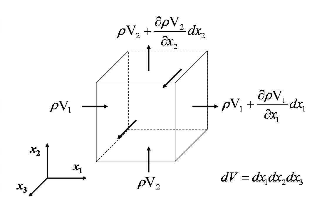
Equating all the mass flow rates into and out of the differential control volume gives
\[ \begin{eqnarray} \rho v_1 (dx_2 dx_3) + \rho v_2 (dx_1 dx_3) + \rho v_3 (dx_1 dx_2) - \left( \rho v_1 + {\partial (\rho v_1) \over \partial x_1} dx_1 \right) dx_2 dx_3 \\ - \left( \rho v_2 + {\partial (\rho v_2) \over \partial x_2} dx_2 \right) dx_1 dx_3 - \left( \rho v_3 + {\partial (\rho v_3) \over \partial x_3} dx_3 \right) dx_1 dx_2 = {\partial \over \partial t} (\rho dx_1 dx_2 dx_3) \end{eqnarray} \]
Cancelling terms and dividing through by \(dx_1 dx_2 dx_3\) gives
\[ \begin{eqnarray} - {\partial (\rho v_1) \over \partial x_1} - {\partial (\rho v_2) \over \partial x_2} - {\partial (\rho v_3) \over \partial x_3} = {\partial \rho \over \partial t} \end{eqnarray} \]
\[ {\partial \rho \over \partial t} + {\partial (\rho v_1) \over \partial x_1} + {\partial (\rho v_2) \over \partial x_2} + {\partial (\rho v_3) \over \partial x_3} = 0 \]
This can be written concisely as
\[ {\partial \rho \over \partial t} + \nabla \cdot (\rho {\bf v}) = 0 \qquad \qquad { \partial \rho \over \partial t} + (\rho \, v_i),_{\,i} = 0 \]
Important Points
These are the final, complete, and most general forms of the continuity equation that enforces conservation of mass. It applies to all materials, not just fluids. So it applies to solids as well. Note that it is a single scalar equation and is Eulerian in nature because the gradient terms are \({\partial \over \partial x_i}\), not \({\partial \over \partial X_i}\).One might wonder if there is a Lagrangian counterpart to the Eulerian form of this. There is. It is usually written as
\[ \rho \, dV = \rho_o dV_o \]
This simply states that the differential chunk of mass in the deformed state \(\rho \, dV\) must be equal to its original value \(\rho_o dV_o\) in the undeformed state.
\[ \nabla \cdot (\rho {\bf v}) = 0 \qquad \qquad (\rho \, v_i),_{\,i} = 0 \qquad \qquad \text{(steady state)} \]
The second special case is that of incompressibility, i.e., \(\rho = \)constant. In this case the derivative with respect to time is zero and \(\rho\) can be factored out of the equation leaving only
\[ \nabla \cdot {\bf v} = 0 \qquad \qquad \quad v_{i,i} = 0 \qquad \qquad \quad \text{(incompressible)} \]
This result is simple enough that it is often expanded out.
\[ {\partial v_1 \over \partial x_1} + {\partial v_2 \over \partial x_2} + {\partial v_3 \over \partial x_3} = 0 \qquad \qquad \qquad \text{(incompressible)} \]
Note that this is nothing more than \(\text{tr}({\bf D}) = 0\) for the case of incompressible materials.
Material Derivative
The following is worth pointing out because it permits the density and velocity vector to be separated. The first step is to apply the product rule to the divergence term in the continuity equation.\[ {\partial \rho \over \partial t} + {\bf v} \cdot \nabla \rho + \rho \, (\nabla \cdot {\bf v}) = 0 \]
And then note that \({\partial \rho \over \partial t} + {\bf v} \cdot \nabla \rho\) is just the material derivative of the density, \({D \rho \over D t}\).
So the continuity equation can also be written as
If the material is incompressible, then \(\rho\) cannot change, so \( {D \rho \over D t} \) must be zero, leaving
\[ \rho \nabla \cdot {\bf v} = 0 \]
And then divide through by \(\rho\) (since it's not zero) to get
\[ \nabla \cdot {\bf v} = 0 \]
Continuity Equation Example

\[ {\partial v_1 \over \partial x_1} + {\partial v_2 \over \partial x_2} = 0 \]
Start by looking at the y-component of the flow, \(v_2\). The geometry of the converging nozzle forces the \(v_2\) component to flow upward when \(y \lt 0\) and flow downward when \(y \gt 0\). So \(v_2 \gt 0\) when \(y \lt 0\) and \(v_2 \lt 0\) when \(y \gt 0\).
The net effect of this is that \( {\partial v_2 \over \partial x_2} \lt 0 \) in the converging nozzle.
But the continuity equation dictates that the sum of the two partial derivatives must equal zero. So if the second is less than zero, then
\[ {\partial v_1 \over \partial x_1} \gt 0 \]
And this means that the fluid flow must be accelerating.