Search Continuum Mechanics Website

Special Strain Topics

 home > deformation & strain > special topics

Introduction

This page looks at the strain states present in a typical tire. Understanding such deformation modes is relevant to knowing how to best perform material tests in the lab to characterize rubber behavior in support of tire design and development. For example, it can be important to know whether a portion of a tire is deforming primarily in uniaxial tension or in shear so that lab tests can be developed to characterize the rubber's strength, stiffness, damping, etc, in the appropriate deformation mode.

The page contains notes I compiled many years ago. So enjoy the old graphics!

---

Deformation States

Any strain state can be transformed to its principal orientation, allowing it to be described by only the three principal strain values, along with its orientation vector, ${\bf Q}$.

Look at the three deformation states below that are described in terms of the principal strains.



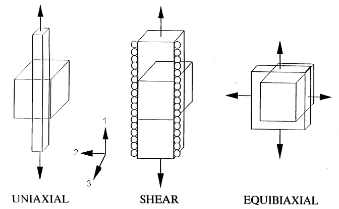
In each case, the cube is being stretched the most in the $1$ direction, and shrinking the most in the $3$ direction. But it is the $2$ direction that dictates the deformation mode. In the tension case at the far left, $\epsilon_2 = \epsilon_3$, both of which are negative.

In the center case, the second principal strain is zero. This is shear in which $\gamma_{\text{Max}} = \epsilon_1 - \epsilon_3$, while the remaining strain, $\epsilon_2$, is zero.

In the far right case, the second principal strain is the maximum possible, which is equal to $\epsilon_1$. This is called equibiaxial tension, although it is in fact the same as compression.

This key here is that it is the middle principal strain, which is bounded between the max and min principals, which is the key to identifying the deformation state.

---

Deformation States and Strain Transformations

If the material is rubber, which is incompressible, then only two of the principal strains are independent. So it is useful to transform the problem from the principal strains to a set of three new parameters such that the third, dependent one, is zero, or at least very close. One way of doing this is through invariants. But invariants are practically impossible to intuitively relate directly to a deformed state (such as uniaxial tension or shear). So an alternative is desirable.

One such alternative is as follows:

$$\left[ \matrix{ \epsilon_1 & 0 & 0 \\ 0 & \epsilon_2 & 0 \\ 0 & 0 & \epsilon_3 } \right] = \epsilon_{\text{Hyd}} \left[ \matrix{ 1 & 0 & 0 \\ 0 & 1 & 0 \\ 0 & 0 & 1 } \right] + (\epsilon_1 - \epsilon_3) \left[ \matrix{ 1/2 & 0 & 0 \\ 0 & 0 & 0 \\ 0 & 0 & -1/2 } \right] + (\epsilon_2 - \epsilon_{\text{Hyd}}) \left[ \matrix{ -1/2 & 0 & 0 \\ 0 & 1 & 0 \\ 0 & 0 & -1/2 } \right]$$
where $\epsilon_1 > \epsilon_2 > \epsilon_3$.

This can be checked by multiplying each term of the matrix out. For example, looking at the $11$ slot gives

$$\begin{eqnarray} \epsilon_1 & = & \epsilon_{\text{Hyd}} + {1 \over 2} ( \epsilon_1 - \epsilon_3 ) - {1 \over 2} (\epsilon_2 - \epsilon_{\text{Hyd}}) \\ \\ & = & {\epsilon_1 + \epsilon_2 + \epsilon_3 \over 3} + {1 \over 2} ( \epsilon_1 - \epsilon_3 ) - {1 \over 2} (\epsilon_2 -{\epsilon_1 + \epsilon_2 + \epsilon_3 \over 3}) \\ \\ & = & \epsilon_1 \end{eqnarray}$$
Doing the same steps for the $22$ and $33$ components will confirm the identities.

The relationship can be simplified somewhat by noting that $\gamma_{\text{Max}} = \epsilon_1 - \epsilon_3$ because $\epsilon_1$ and $\epsilon_3$ are the max and min principal strains.

Likewise, ($\epsilon_2 - \epsilon_{\text{Hyd}}$) can be named $\gamma_{\text{Secondary}}$ because its matrix is traceless, so it is a shear condition.

So the equation can be written a little more concisely as

$$\left[ \matrix{ \epsilon_1 & 0 & 0 \\ 0 & \epsilon_2 & 0 \\ 0 & 0 & \epsilon_3 } \right] = \epsilon_{\text{Hyd}} \left[ \matrix{ 1 & 0 & 0 \\ 0 & 1 & 0 \\ 0 & 0 & 1 } \right] + \gamma_{\text{Max}} \left[ \matrix{ 1/2 & 0 & 0 \\ 0 & 0 & 0 \\ 0 & 0 & -1/2 } \right] + \gamma_{\text{Sec}} \left[ \matrix{ -1/2 & 0 & 0 \\ 0 & 1 & 0 \\ 0 & 0 & -1/2 } \right]$$
For uniaxial tension, $\epsilon_2 = \epsilon_3$, so

$$\epsilon_{\text{Hyd}} = {\epsilon_1 + 2 \epsilon_3 \over 3}$$
and

$$\begin{eqnarray} \gamma_{\text{Sec}} & = & \epsilon_2 - \epsilon_{\text{Hyd}} \\ \\ & = & \epsilon_3 - {\epsilon_1 + 2 \epsilon_3 \over 3} \\ \\ & = & {\epsilon_3 - \epsilon_1 \over 3} \end{eqnarray}$$
This is exactly -1/3 of $\gamma_{\text{Max}}$, so

$$\text{Uniaxial Tension:} \qquad {\gamma_{\text{Sec}} \over \gamma_{\text{Max}} } = - {1 \over 3}$$
At the other extreme is the case of equibiaxial tension. In this case, $\epsilon_2 = \epsilon_1$, so

$$\epsilon_{\text{Hyd}} = {2 \epsilon_1 + \epsilon_3 \over 3}$$
and

$$\begin{eqnarray} \gamma_{\text{Sec}} & = & \epsilon_2 - \epsilon_{\text{Hyd}} \\ \\ & = & \epsilon_1 - {2 \epsilon_1 + \epsilon_3 \over 3} \\ \\ & = & {\epsilon_1 - \epsilon_3 \over 3} \end{eqnarray}$$
This is exactly 1/3 of $\gamma_{\text{Max}}$, so

$$\text{Equibiaxial Tension:} \qquad {\gamma_{\text{Sec}} \over \gamma_{\text{Max}} } = {1 \over 3}$$
The shear state actually depends on which strain tensor is being used. If it is true strain, then $\gamma_{\text{Sec}} / \gamma_{\text{Max}} = 0$ is exactly pure shear. For Green strain, the ratio for pure shear drifts slightly negative at large strains. It equals $-\gamma_{\text{Max}}/12$.

Nevertheless, the ratio $\gamma_{\text{Sec}} / \gamma_{\text{Max}}$ varies from -1/3 to +1/3 and completely characterizes the deformation state.

---

Deformation States in a Tire

So now let's take a look at the conditions in a tire. It is a 205/70R14 XW4 (from long ago). And element #128 is in the shoulder of the tire. It is rolling straight ahead at nominal load and pressure. (Everything below is based on Green strains.)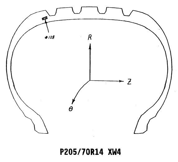



The strain components, in cylindrical components, in the shoulder (element #128) are shown below as a function of angle around the tire.



It is hard to tell in the above graphs just what the deformation state(s) is. But this can be made clearer by transforming the strains into principals and calculating $\gamma_{\text{Max}}$ and $\gamma_{\text{Sec}}$.



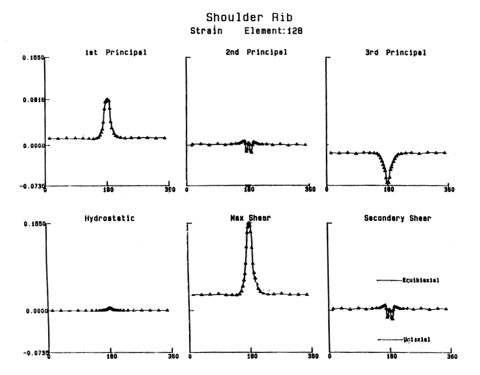
The graphs show that this portion of the shoulder actually spends the majority of its time in shear as it passes through the contact patch because $\gamma_{\text{Sec}}$ does not approach $\pm \gamma_{\text{Max}}/3$.

In fact, the next graph shows that the majority of the tire is in shear in the contact patch.



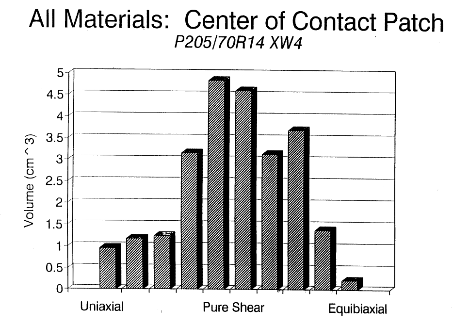
Here is the tread at the center of the contact patch. It has the highest fraction of material undergoing uniaxial tension.



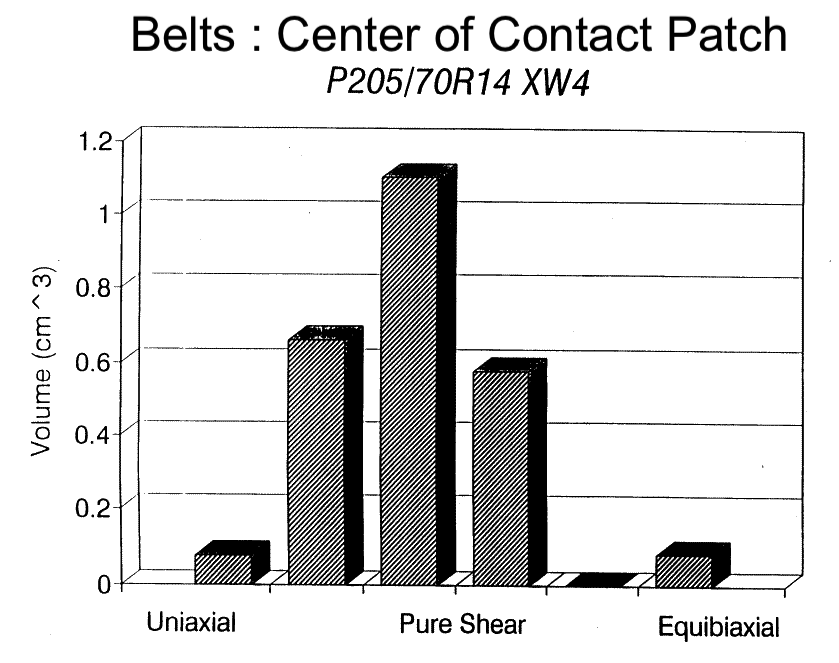
And here are the belts. Back to shear. Probably coming from intercable shear and belt edge shear.



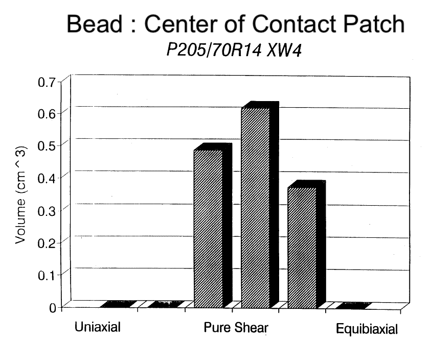
And here is the bead. Definitely shear.



And finally the entire cross-section opposite the contact patch.



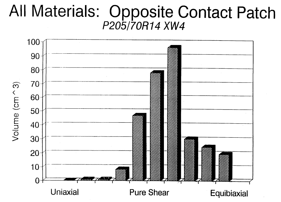
These examples have shown that rubber in the XW4 passenger tire deforms predominantly in shear.