Introduction
This page is all about \(\sum {\bf F} = m \, {\bf a}\), except we will express the forces as stresses acting on differential sized areas. The first example will be 2-D, to minimize the complexity. Then the equations will be developed in 3-D, and also presented in cylindrical coordinates.Following development of the equations, applications will be presented that involve Airy stress functions and tire mechanics. Finally, the equilibrium equations are used to develop expressions for the speed of stress waves in steel, aluminum, and rubber.
2-D Equilibrium
The 2-D differential object is shown in the sketch at the right. The idea is to sum all the forces on it and set them equal to \(m \, {\bf a}\). This can be done one component at a time, so start with the x-direction. The forces consist of
- \(\sigma_{xx}\) acting on face \(dy\) in the \(-x\) direction
- \(\tau_{xy}\) acting on face \(dx\) in the \(-x\) direction
- \(\sigma_{xx} + {\partial \sigma_{xx} \over \partial x} dx\) acting on face \(dy\) in the \(+x\) direction
- \(\tau_{xy} + {\partial \tau_{xy} \over \partial y} dy\) acting on face \(dx\) in the \(+x\) direction
- Plus "body forces". These include any forces due to gravity, magnetism, etc, and are summarized simply as \(\rho f_x dx dy\) where \(f_x\) is force per unit mass
Acceleration is simply \(a_x\), although it is perfectly permissible to use the material derivative: \({\partial v_x \over \partial t} + v_x {\partial v_x \over \partial x} + v_y {\partial v_x \over \partial y} \).
Summing all this up gives
\[ -\sigma_{xx}dy - \tau_{xy}dx + \left( \sigma_{xx} + {\partial \sigma_{xx} \over \partial x} dx \right) dy + \left( \tau_{xy} + {\partial \tau_{xy} \over \partial y} dy \right) dx + \rho f_x dx dy = \rho \, dx dy \, a_x \]
Cleaning up terms that cancel, and dividing through by \(dx dy\) gives
\[ {\partial \sigma_{xx} \over \partial x} + {\partial \tau_{xy} \over \partial y} + \rho f_x = \rho \, a_x \]
And summing forces in the y-direction leads to
\[ {\partial \sigma_{yy} \over \partial y} + {\partial \tau_{xy} \over \partial x} + \rho f_y = \rho \, a_y \]
It is interesting how the equations tie together changes in all the different stress components, making them interdependent on each other.
An object is said to be in equilibrium when the right hand sides (RHS) of the equations are zero.
3-D Equilibrium
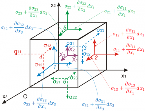
The forces consist of
- \(\sigma_{11}\) acting on face \(dx_2 dx_3\) in the \(-x_1\) direction
- \(\sigma_{21}\) acting on face \(dx_1 dx_3\) in the \(-x_1\) direction
- \(\sigma_{31}\) acting on face \(dx_1 dx_2\) in the \(-x_1\) direction
- \(\sigma_{11} + {\partial \sigma_{11} \over \partial x_1} dx_1\) acting on face \(dx_2 dx_3\) in the \(+x_1\) direction
- \(\sigma_{21} + {\partial \sigma_{21} \over \partial x_2} dx_2\) acting on face \(dx_1 dx_3\) in the \(+x_1\) direction
- \(\sigma_{31} + {\partial \sigma_{31} \over \partial x_3} dx_3\) acting on face \(dx_1 dx_2\) in the \(+x_1\) direction
- The body force is \(\rho f_x dx_1 dx_2 dx_3\) where \(f_1\) is force per unit mass
The mass is density times volume: \(\rho \, dx_1 dx_2 dx_3\).
Acceleration is simply \(a_1\), although it is perfectly permissible to use the material derivative: \({\partial v_1 \over \partial t} + v_1 {\partial v_1 \over \partial x_1} + v_2 {\partial v_1 \over \partial x_2} + v_3 {\partial v_1 \over \partial x_3}\).
Summing all this up gives
\[ {\partial \sigma_{11} \over \partial x_1} dx_1 dx_2 dx_3 + {\partial \sigma_{21} \over \partial x_2} dx_1 dx_2 dx_3 + {\partial \sigma_{31} \over \partial x_3} dx_1 dx_2 dx_3 + \rho f_1 = \rho \, dx_1 dx_2 dx_3 a_1 \]
Dividing through by the differential volumes gives
\[ {\partial \sigma_{11} \over \partial x_1} + {\partial \sigma_{21} \over \partial x_2} + {\partial \sigma_{31} \over \partial x_3} + \rho f_1 = \rho \, a_1 \]
And since the stress tensor is symmetric...
\[ {\partial \sigma_{11} \over \partial x_1} + {\partial \sigma_{12} \over \partial x_2} + {\partial \sigma_{13} \over \partial x_3} + \rho f_1 = \rho \, a_1 \]
The complete set of equations is
\[ {\partial \sigma_{11} \over \partial x_1} + {\partial \sigma_{12} \over \partial x_2} + {\partial \sigma_{13} \over \partial x_3} + \rho f_1 = \rho \, a_1 \] \[ {\partial \sigma_{21} \over \partial x_1} + {\partial \sigma_{22} \over \partial x_2} + {\partial \sigma_{23} \over \partial x_3} + \rho f_2 = \rho \, a_2 \] \[ {\partial \sigma_{31} \over \partial x_1} + {\partial \sigma_{32} \over \partial x_2} + {\partial \sigma_{33} \over \partial x_3} + \rho f_3 = \rho \, a_3 \]
All this is written in matrix and tensor notation as
\[ \nabla \cdot \boldsymbol{\sigma} + \rho \, {\bf f} = \rho \, {\bf a} \qquad \qquad \sigma_{ij,j} + \rho f_i = \rho \, a_i \]
Or one could write the acceleration as the material derivative.
\[ \nabla \cdot \boldsymbol{\sigma} + \rho \, {\bf f} = \rho \, \left( {\partial {\bf v} \over \partial t} + {\bf v} \cdot {\partial {\bf v} \over \partial {\bf x}} \right) \qquad \qquad \sigma_{ij,j} + \rho f_i = \rho \, ( v_{i,t} + v_k v_{i,k} ) \]
Equilibrium in Cylindrical Coordinates
The equilibrium equations in cylindrical coordinates contain several additional terms, such as \({\sigma_{\theta \theta} \over r}\) and \({\sigma_{\theta z} \over r}\), that further complicate matters.\[ \begin{eqnarray} & & {1 \over r} {\partial \over \partial \, r} \left( r \sigma_{rr} \right) + {1 \over r} {\partial \, \sigma_{\!r\theta} \over \partial \, \theta} + {\partial \, \sigma_{\!rz} \over \partial z} - { \sigma_{\!\theta\theta} \over r} + \rho f_r = \rho \, a_r \\ \\ \\ & & {1 \over r} {\partial \over \partial \, r} \left( r \sigma_{r \theta} \right) + {1 \over r} {\partial \, \sigma_{\!\theta\theta} \over \partial \, \theta} + {\partial \, \sigma_{\!\theta z} \over \partial z} + {\sigma_{\!r \theta} \over r} + \rho f_\theta = \rho \, a_\theta \\ \\ \\ & & {1 \over r} {\partial \over \partial \, r} \left( r \sigma_{rz} \right) + {1 \over r} {\partial \, \sigma_{\!\theta z} \over \partial \, \theta} + {\partial \, \sigma_{\!zz} \over \partial z} + \rho f_z = \rho \, a_z \end{eqnarray} \]
Centripetal Acceleration
It is possible to get a quick, rough estimate of the circumferential stress level in a tire undergoing axisymmetric centripetal forces during a high speed limit test. The radial acceleration equation is\[ {1 \over r} {\partial \over \partial \, r} \left( r \sigma_{rr} \right) + {1 \over r} {\partial \, \sigma_{\!r\theta} \over \partial \, \theta} + {\partial \, \sigma_{\!rz} \over \partial z} - { \sigma_{\!\theta\theta} \over r} + \rho f_r = \rho \, a_r \\ \]
The radial acceleration is
\[ a_r = - {V^2 \over r} \]
The other terms are expected to be negligible, except \(\sigma_{\theta\theta} / r\). Setting these two equal to each other gives
\[ - {\sigma_{\theta\theta} \over r} = - \rho {V^2 \over r} \]
This simplifies to
\[ \sigma_{\theta\theta} = \rho V^2 \]
So for a tire spinning at 200 kph (= 55.55 m/s), with rubber density equal to 1,150 kg/m3, the circumferential stress should be around
\[ \sigma_{\theta\theta} \; = \; (1150 \text{ kg/m}^3) (55.55 \text{ m/s})^2 \; = \; 3,500,000 \text{ Pa} \; = \; 3.5 \text{ MPa} \]
For the steel in the NSTs, the density is 7,800 kg/m3, and the circumferential stress should be around
\[ \sigma_{\theta\theta} \; = \; (7800 \text{ kg/m}^3) (55.55 \text{ m/s})^2 \; = \; 24,000,000 \text{ Pa} \; = \; 24 \text{ MPa} \]
The fact that the tire is actually a nonhomogeneous composite probably makes the actual values significantly different from these estimates.
Steel Belt Equilibrium
This example relates interply shear strain, \(\gamma_{xz}\), which is present between the steel belts and peaks at the belt edge, to intraply shear stress, \(\tau_{xy}\), in the plane of the belts.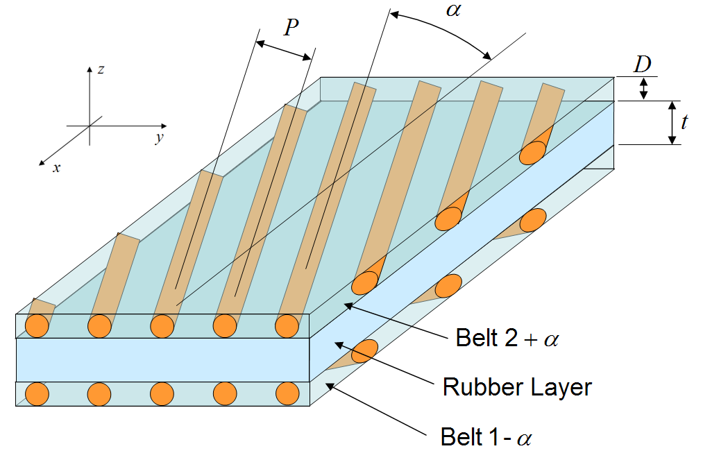
The main governing equilibrium equation for this situation is
\[ {\partial \sigma_{xx} \over \partial x} + {\partial \tau_{xy} \over \partial y} + {\partial \tau_{xz} \over \partial z} + \rho f_x = \rho \, a_x \]
Assume that several terms in the equation are negligible, leaving only
\[ {\partial \tau_{xy} \over \partial y} + {\partial \tau_{xz} \over \partial z} = 0 \]
The interply rubber layer develops shear, called \(\gamma_{xz}\). Therefore the shear stress is
\[ \tau_{xz} = G \gamma_{xz} \]
Now focus on the top belt. The shear stress, \(\tau_{xz}\), in the shear layer is the shear stress on the bottom surface of the belt. But the shear stress on the top is near zero. So the change in shear stress through the thickness of the belt is
\[ {\partial \tau_{xz} \over \partial z} \; = \; {\tau_\text{top} - \tau_\text{bottom} \over D} \; = \; {0 - G \gamma_{xz} \over D} \; = \; -\left( { G \over D}\right) \gamma_{xz} \]
\[ {\partial \tau_{xy} \over \partial y} - \left( { G \over D}\right) \gamma_{xz} = 0 \]
So the intraply shear in the belt can be related to the interply shear strain as
\[ \tau_{xy} = \int \left( { G \over D}\right) \gamma_{xz} \, dy \]
Granted, this equation my not be very useful by itself. But it is essential to the general analytical solution for the stresses and strains in the belts.
Airy Stress Functions
The use of Airy Stress Functions is a powerful technique for solving 2-D equilibrium elasticity problems. The approach will be presented here for the special case of no body forces.First, note that in 2-D equilibrium (\({\bf a} = 0\)), and in the absence of body forces (\({\bf f} = 0\)), the equilbrium equations reduce to
\[ {\partial \sigma_{xx} \over \partial x} + {\partial \tau_{xy} \over \partial y} = 0 \qquad \qquad {\partial \sigma_{yy} \over \partial y} + {\partial \tau_{xy} \over \partial x} = 0 \]
Next, propose that a scalar function, \(\phi\), exists (the Airy stress function) and is related to the 2-D stress components by the following cleverly chosen relationships.
\[ \sigma_{xx} = {\partial^2 \phi \over \partial y^2} \qquad \sigma_{yy} = {\partial^2 \phi \over \partial x^2} \qquad \tau_{xy} = - {\partial^2 \phi \over \partial x \partial y} \]
Then, substituting the above \(\phi\) relationships into the equilibrium equations gives a remarkable result.
\[ {\partial \over \partial x} \left( {\partial^2 \phi \over \partial y^2} \right) - {\partial \over \partial y} \left( {\partial^2 \phi \over \partial x \partial y} \right) = 0 \] \[ {\partial \over \partial y} \left( {\partial^2 \phi \over \partial x^2} \right) - {\partial \over \partial x} \left( {\partial^2 \phi \over \partial x \partial y} \right) = 0 \]
The remarkable result here is that the equilibrium equations are always satisfied regardless of the choice of \(\phi\). So any choice of \(\phi\) is the solution to a problem (well almost, more on this in a moment). But which problem? Indeed, when one works with Airy stress functions, one can find oneself with a solution, but not know what problem it is a solution to!
Take for example, \(\phi = {1 \over 2} A y^2\). This is the solution to something. But what? To find out, take the partial derivatives to determine the stress fields. This leads to
\[ \sigma_{xx} \; = \; {\partial^2 \over \partial y^2} \left( {1 \over 2} A y^2 \right) \; = \; A \]
Therefore, this is easily recognized as a simple case of uniaxial tension in the \(x\) direction. Likewise, letting \(\phi = -B x y\) leads to a state of uniform pure shear in which \(\tau_{xy} = B\).
It is perhaps worth noting that Airy stress functions have been used extensively in the field of Fracture Mechanics.
Nevertheless, nothing is quite THAT easy. There is one limitation on the choice of \(\phi\) that results from the facts that the solutions are restricted to isotropic materials, the strains are related to stresses through Hooke's Law, and they must make physical sense, e.g., the strains cannot be so negative that the material folds back on itself. The limitation is that \(\phi\) must satisfy the Biharmonic Equation. It is
\[ {\partial^4 \phi \over \partial x^4} + 2 {\partial^4 \phi \over \partial x^2 \partial y^2} + {\partial^4 \phi \over \partial y^4} = 0 \]
and is abbreviated \(\nabla^4 \phi = 0\). It is not at all intuitive why the restrictions lead to the biharmonic equation, and there is a great deal of tedious algrebra required to show it, but it is indeed the case. Any \(\phi\) function satisfying \(\nabla^4 \phi = 0\) is guaranteed to produce stress and strain fields that are in equilibrium for an isotropic solid not subjected to body forces.
Note that any polynomial of degree 3 or less in \(x\) and \(y\) is automatically a solution of the biharmonic equation because the equation contains 4th order derivatives.
Polar Coordinates
In polar coordinates, the biharmonic equation is\[ \left( {1 \over r} {\partial \over \partial r} \left( r \, {\partial \over \partial r} \right) + {1 \over r^2} {\partial^2 \over \partial \theta^2} \right)^2 \phi = 0 \]
and the relationships for the stress components are
\[ \sigma_{rr} = {1 \over r} {\partial \phi \over \partial r} + {1 \over r^2} {\partial^2 \phi \over \partial \theta^2} \qquad \qquad \sigma_{\theta \theta} = {\partial^2 \phi \over \partial r^2} \qquad \qquad \tau_{r \theta} = - {\partial \over \partial r} \left( {1 \over r} {\partial \phi \over \partial \theta} \right) \]
Line Load Example
The case of a distributed linear load \(P'\) on an infinite solid can be solved with Airy stress functions in polar coordinates. The stress function in this case is
\[ \phi = - {P' \over \pi} r \, \theta \cos \theta \]
The function can be inserted in the biharmonic equation to verify that it is indeed a solution. The stress components obtained from differentiating the stress function are therefore a valid solution to a particular problem. But which one? To determine that, first evaluate the stresses.
\[ \begin{eqnarray} \sigma_{rr} & = & {1 \over r} {\partial \phi \over \partial r} + {1 \over r^2} {\partial^2 \phi \over \partial \theta^2} \\ \\ & = & - {2 \, P' \over \pi \, r} \cos \theta \\ \\ \\ \sigma_{\theta \theta} & = & {\partial^2 \phi \over \partial r^2} \; = \; 0 \\ \\ \\ \tau_{r \theta} & = & - {\partial \over \partial r} \left( {1 \over r} {\partial \phi \over \partial \theta} \right) \; = \; 0 \end{eqnarray} \]
This stress field results from a distributed line load of zero width. This can be varified by computing the net vertical force due to the radial stress using
\[ \begin{eqnarray} \text{Vertical Load / Length} & = & - \int_{-\pi/2}^{\pi/2} \sigma_{rr} \cos \theta \, r d \theta \qquad \qquad \quad \end {eqnarray} \]
where the \(\cos \theta\) term gives the vertical component of force due to the radial stress. Substituting the expression for \(\sigma_{rr}\) into the equation and integrating gives
\[ \begin{eqnarray} \text{Vertical Load / Length} & = & - \int_{-\pi/2}^{\pi/2} \left( - {2 \, P' \over \pi \, r} \cos \theta \right) \cos \theta \, r d \theta \\ \\ & = & {2\, P' \over \pi} \int_{-\pi/2}^{\pi/2} \cos^2 \theta \; d \theta \\ \\ & = & P' \end{eqnarray} \]
Equilibrium and the Speed of Stress Waves
\[ {\partial^2 u \over \partial x^2} = {1 \over c^2} {\partial^2 u \over \partial t^2} \]
where \(u\) represents displacement, and \(c\) is the speed of the stress waves in the material - effectively the speed of sound in the material. (And this is the focus of this discussion.)
Now bring up the following equilibrium equation
\[ {\partial \sigma_{xx} \over \partial x} + {\partial \tau_{xy} \over \partial y} + {\partial \tau_{xz} \over \partial z} + \rho f_x = \rho \, a_x \]
and neglect the shear and body force terms, leaving only
\[ {\partial \sigma_{xx} \over \partial x} = \rho \, a_x \]
And now substitute several relationships. Begin by noting that \(a_x = {\partial^2 u \over \partial t^2}\) just like in the wave equation.
Next, note that \(\sigma_{xx}\) in the equilibrium equation is related to \(\epsilon_{xx}\) by
\[ \sigma_{xx} = E \epsilon_{xx} \]
for the case of uniaxial tension. But then, \(\epsilon_{xx}\) is related to the displacements through
\[ \epsilon_{xx} = {\partial u \over \partial x} \]
Again, this is for the simple case of uniaxial tension. So stress can be related to displacements by
\[ \sigma_{xx} \; = \; E \epsilon_{xx} \; = \; E {\partial u \over \partial x} \]
And
\[ {\partial \sigma_{xx} \over \partial x} = E {\partial^2 u \over \partial x^2} \]
Substituting all this into the equilibrium equation gives
\[ E {\partial^2 u \over \partial x^2} = \rho {\partial^2 u \over \partial t^2} \]
\[ {\partial^2 u \over \partial x^2} = {1 \over (E/\rho)} {\partial^2 u \over \partial t^2} \]
Now the big finish.... Comparing this to the wave equation shows that
\[ c^2 = {E \over \rho} \qquad \quad \text{or} \quad \qquad c = \sqrt{E \over \rho} \]
And that is the relationship for the speed of a uniaxial stress wave through a material, its speed of sound!
Speed of Sound in Materials
For steel, \(E = 200(10)^9 \text{ Pa}\) and \(\rho = 7,800 \text{ kg/m}^3\). So this gives\[ c \; = \; \sqrt{E \over \rho} \; = \; \sqrt{200(10)^9 \text{ Pa} \over 7,800 \text{ kg/m}^3} \; = \; 5 \text{ km/s} \; = \; 5 \text{ m/ms} \]
For aluminum, \(E = 70(10)^9 \text{ Pa}\) and \(\rho = 2,800 \text{ kg/m}^3\). So this gives
\[ c \; = \; \sqrt{E \over \rho} \; = \; \sqrt{70(10)^9 \text{ Pa} \over 2,800 \text{ kg/m}^3} \; = \; 5 \text{ km/s} \; = \; 5 \text{ m/ms} \]
By coincidence, the speed of sound through both steel and aluminum is the same.
For rubber with \(E = 1(10)^6 \text{ Pa}\) and \(\rho = 1,150 \text{ kg/m}^3\). So this gives
\[ c \; = \; \sqrt{E \over \rho} \; = \; \sqrt{1(10)^6 \text{ Pa} \over 1,150 \text{ kg/m}^3} \; = \; 29 \text{ m/s} \; = \; 0.03 \text{ m/ms} \]
Shear Wave Speeds
But we're not done! Take a look at shear waves. This time, bring up the following equilibrium equation\[ {\partial \tau_{yx} \over \partial x} + {\partial \sigma_{yy} \over \partial y} + {\partial \tau_{yz} \over \partial z} + \rho f_y = \rho \, a_y \]
and neglect all the terms except
\[ {\partial \tau_{yx} \over \partial x} = \rho \, a_y \]
And swap the subscripts on \(\tau\) since it's symmetric.
Begin by substituting \(a_y = {\partial^2 v \over \partial t^2}\) just like in the wave equation.
And relate \(\tau_{xy}\) to \(\gamma_{xy}\) by
\[ \tau_{xy} = G \gamma_{xy} \]
And relate \(\gamma_{xy}\) to the displacements with the simple-shear assumption.
\[ \gamma_{xy} = {\partial v \over \partial x} \]
So the shear stress can be related to displacements by
\[ \tau_{xy} \; = \; G \gamma_{xy} \; = \; G {\partial v \over \partial x} \]
And
\[ {\partial \tau_{xy} \over \partial x} = G {\partial^2 v \over \partial x^2} \]
Substituting all this into the equilibrium equation gives
\[ G {\partial^2 v \over \partial x^2} = \rho {\partial^2 v \over \partial t^2} \]
Or
\[ {\partial^2 v \over \partial x^2} = {1 \over (G/\rho)} {\partial^2 v \over \partial t^2} \]
Comparing this to the wave equation shows that
\[ c^2 = {G \over \rho} \qquad \quad \text{or} \quad \qquad c = \sqrt{G \over \rho} \]
So for shear waves their speed depends on the shear modulus, \(G\), not the elongation modulus, \(E\). For incompressible materials, i.e., rubber, the shear modulus is one-third of the tension modulus, so shear waves propagate through rubber at \(1 / \sqrt{3}\), or 58% of the speed of uniaxial tension waves. For metals, the shear modulus is about 38% of the tension modulus. This translates to their shear wave speeds being 61% of their tension wave speeds.
Plane Wave Speeds
And finally, there are plane wave speeds. These are cases where the cross-sections of the objects are very large and hold the lateral strains constant at zero while the object undergoes tension/compression. This doesn't really apply to rubber because volume changes are involved.\[ \sigma_{ij} = {E \over (1 + \nu)} \left[ \epsilon_{ij} + { \nu \over (1 - 2 \nu)} \delta_{ij} \epsilon_{kk} \right] \]
and impose the following: \(\epsilon_{11} = \epsilon\), and \(\epsilon_{22} = \epsilon_{33} = 0\). This gives
\[ \sigma = {E \over (1 + \nu)} \left[ \epsilon + { \nu \over (1 - 2 \nu)} \epsilon \right] \]
which simplifies to
\[ \sigma = {E \, (1 - \nu) \over (1 + \nu) (1 - 2 \nu)} \epsilon \]
You can see that for rubber with \(\nu = 0.5\), the stress required to generate any strain is infinite due to the \((1 - 2 \nu)\) term in the denominator. This is because rubber is incompressible.
As before, substitute \( {\partial u \over \partial x} \) for \(\epsilon\). This gives
\[ \sigma = {E \, (1 - \nu) \over (1 + \nu) (1 - 2 \nu)} {\partial u \over \partial x} \]
And
\[ {\partial \sigma \over \partial x} = {E \, (1 - \nu) \over (1 + \nu) (1 - 2 \nu)} {\partial^2 u \over \partial x^2} \]
Combining everything gives
\[ {E \, (1 - \nu) \over (1 + \nu) (1 - 2 \nu)} {\partial^2 u \over \partial x^2} = \rho {\partial^2 u \over \partial t^2} \]
So the wave speed of plane waves is
\[ c = \sqrt{ { (1 - \nu) \over (1 + \nu) (1 - 2 \nu)} \left( {E \over \rho} \right) } \]
So for metals with \(\nu = 1/3\), the plane wave speed is 22% greater than the uniaxial tension case. And for incompressible rubber with \(\nu = 1/2\), the speed would theoretically be infinite, which is of course impossible. This occurs because compression from a plane wave must result in a volume change, which would theoretically propagate at infinite speed in an incompressible material.
This is resolved by recalling from Hooke's Law that rubber is actually compressible and its bulk modulus is approximately 1,000 MPa. For the plane wave, \(\sigma_{xx} = K \epsilon_{xx}\) because \(\epsilon_{yy} = \epsilon_{zz} = 0\). This leads to
\[ c = \sqrt{ K \over \rho } \]
This produces a plane wave speed in rubber of approximately
\[ c \; = \; \sqrt{K \over \rho} \; = \; \sqrt{1,000\text{E}6 \text{ Pa} \over 1,150 \text{ kg/m}^3} \; = \; 930 \text{ m/s} \; = \; 0.93 \text{ m/ms} \]
Keep in mind that this is only an approximation based on an estimate of the bulk modulus. Nevertheless, the speed is still much less than that in metals.