Introduction
The previous page on small strains demonstrated that their actual limitation is not small strains at all, but rather small rotations. It was demonstrated that as the amount of rotation grows, so does the inaccuracies in the small strain tensor.It was also demonstrated that the stretch tensor, specifically \({\bf U} - {\bf I}\), fulfills all the desired properties of a strain tensor and is not limited to small rotations. However, \({\bf U}\) is very difficult to compute (see this page on polar decompositions), so an alternative strain definition is needed that is easy to calculate and is not corrupted by rigid body rotations. The answer to this dilemma is the Green strain tensor.
Green Strain Definition
The Green strain tensor, \({\bf E}\), is based on the deformation gradient as follows.\[ {\bf E} = {1 \over 2} \left( {\bf F}^T \cdot {\bf F} - {\bf I} \right) \]
Recall that \({\bf F}^T \cdot {\bf F}\) completely eliminates the rigid body rotation, \({\bf R}\), from the problem because
\[ {\bf F}^T \! \cdot {\bf F} \quad = \quad \left( {\bf R} \cdot {\bf U} \right)^T \cdot \left( {\bf R} \cdot {\bf U} \right) \quad = \quad {\bf U}^T \! \cdot {\bf R}^T \cdot {\bf R} \cdot {\bf U} \quad = \quad {\bf U}^T \! \cdot {\bf U} \]
And this leaves only the stretch tensor, \({\bf U}\), in the calculation, confirming that the result is indeed independent of any rotations (you will get the same computed strain regardless of the amount of rotation).
The Green strain tensor, in tensor notation, is
\[ E_{ij} = {1 \over 2} \left( F_{ki} F_{kj} - \delta_{ij} \right) \]
and since \(F_{ij} = \delta_{ij} + u_{i,j}\), then
\[ \begin{eqnarray} E_{ij} & = & {1 \over 2} \left[ (\delta_{ki} + u_{k,i}) (\delta_{kj} + u_{k,j}) - \delta_{ij} \right] \\ \\ \\ & = & {1 \over 2} \left[ \delta_{ki} \delta_{kj} + \delta_{ki} u_{k,j} + \delta_{kj} u_{k,i} + u_{k,i} u_{k,j} - \delta_{ij} \right] \\ \\ \\ & = & {1 \over 2} \left[ \delta_{ij} + u_{i,j} + u_{j,i} + u_{k,i} u_{k,j} - \delta_{ij} \right] \\ \\ \\ & = & {1 \over 2} \left[ u_{i,j} + u_{j,i} + u_{k,i} u_{k,j} \right] \end{eqnarray} \]
\[ E_{ij} = {1 \over 2} \left( {\partial \, u_i \over \partial X_j} + {\partial \, u_j \over \partial X_i} + {\partial \, u_k \over \partial X_i} {\partial \, u_k \over \partial X_j} \right) \]
The strain tensor, which is symmetric, is
\[ {\bf E} = \left[ \matrix{ E_{xx} & E_{xy} & E_{xz} \\ \\ E_{xy} & E_{yy} & E_{yz} \\ \\ E_{xz} & E_{yz} & E_{zz} } \right] \]
The specific expressions for each component of the Green strain tensor are listed here. Keep in mind that \({\bf u} = (u,v,w)\).
\[ \begin{eqnarray} E_{xx} & = & {\partial \, u \over \partial X} + {1 \over 2} \left[ \left( {\partial \, u \over \partial X} \right)^2 + \left( {\partial \, v \over \partial X} \right)^2 + \left( {\partial \, w \over \partial X} \right)^2 \right] \\ \\ \\ E_{yy} & = & {\partial \, v \over \partial Y} + {1 \over 2} \left[ \left( {\partial \, u \over \partial Y} \right)^2 + \left( {\partial \, v \over \partial Y} \right)^2 + \left( {\partial \, w \over \partial Y} \right)^2 \right] \\ \\ \\ E_{zz} & = & {\partial \, w \over \partial Z} + {1 \over 2} \left[ \left( {\partial \, u \over \partial Z} \right)^2 + \left( {\partial \, v \over \partial Z} \right)^2 + \left( {\partial \, w \over \partial Z} \right)^2 \right] \\ \\ \\ E_{xy} & = & {1 \over 2} \left( {\partial \, u \over \partial Y} + {\partial \, v \over \partial X} \right) + {1 \over 2} \left[ {\partial \, u \over \partial X} {\partial \, u \over \partial Y} + {\partial \, v \over \partial X} {\partial \, v \over \partial Y} + {\partial \, w \over \partial X} {\partial \, w \over \partial Y} \right] \\ \\ \\ E_{xz} & = & {1 \over 2} \left( {\partial \, u \over \partial Z} + {\partial \, w \over \partial X} \right) + {1 \over 2} \left[ {\partial \, u \over \partial X} {\partial \, u \over \partial Z} + {\partial \, v \over \partial X} {\partial \, v \over \partial Z} + {\partial \, w \over \partial X} {\partial \, w \over \partial Z} \right] \\ \\ \\ E_{yz} & = & {1 \over 2} \left( {\partial \, v \over \partial Z} + {\partial \, w \over \partial Y} \right) + {1 \over 2} \left[ {\partial \, u \over \partial Y} {\partial \, u \over \partial Z} + {\partial \, v \over \partial Y} {\partial \, v \over \partial Z} + {\partial \, w \over \partial Y} {\partial \, w \over \partial Z} \right] \\ \end{eqnarray} \]
The equations are certainly too complex to provide much intuitive insight into their properties, other than the fact that it is known that they are independent of rotations. Perhaps the best insight is that they can be grouped into...
\[ \text{Green Strain = Small Strain Terms + Quadratic Terms} \]
The small strain terms are the same, possessing all the desirable properties of engineering strain behavior. The quadratic terms are what gives the Green strain tensor its rotation independence. But this does come at a price, the \(\epsilon = \Delta L / L_o\) and \(\gamma = D / T\) behaviors are affected by the quadratic terms when the strains are large. (Not just rotations this time, but actual strains.) This is discussed in more detail shortly.
Shear Term Alert
Do not forget that the shear terms are one half of the engineering shear values because they are components in a strain tensor!U - I, Small Strain, Green Strain
Recall this example from the small strain page. The deformation gradient, \({\bf F}\), is written below. And recall that it corresponds to a 25° rigid body rotation about \({\bf p} = (-0.0404,-0.3539,-0.8859)\).\[ {\bf F} = \left[ \matrix{ 1 & 0.495 & 0.5 \\ -0.333 & 1 & -0.247 \\ \;\;\; 0.959 & 0 & 1.5 } \right] \]
The rotation matrix, \({\bf R}\), and stretch tensor, \({\bf U}\), are:
\[ {\bf R} = \left[ \matrix{ \;\;\;0.903 & 0.378 & -0.140 \\ -0.368 & 0.925 & \;\;\;0.045 \\ \;\;\;0.158 & 0.011 & \;\;\;0.986 } \right] \qquad {\bf U} = \left[ \matrix{ 1.195 & \;\;\;0.078 & \;\;\;0.779 \\ 0.078 & \;\;\;1.113 & -0.024 \\ 0.779 & -0.024 & \;\;\;1.396 } \right] \]
The small strain tensor: \(\boldsymbol{\epsilon} = \frac{1}{2} ({\bf F} + {\bf F}^T) - {\bf I}\), and \({\bf U} - {\bf I}\) are
\[ \boldsymbol{\epsilon} = \left[ \matrix{ 0.000 & \;\;\;0.081 & \;\;\;0.730 \\ 0.081 & \;\;\;0.000 & -0.124 \\ 0.730 & -0.124 & \;\;\;0.500 } \right] \qquad {\bf U} - {\bf I} = \left[ \matrix{ 0.195 & \;\;\;0.078 & \;\;\;0.779 \\ 0.078 & \;\;\;0.113 & -0.024 \\ 0.779 & -0.024 & \;\;\;0.396 } \right] \]
\[ {\bf E} = \left[ \matrix{ 0.515 & 0.081 & 1.010 \\ 0.081 & 0.123 & 0.000 \\ 1.010 & 0.000 & 0.781 } \right] \]
which is different still from both the small strain tensor, \(\boldsymbol{\epsilon}\), and \({\bf U} - {\bf I}\). But while \(\boldsymbol{\epsilon}\) will change with rotation, at least \({\bf E}\) does not. This is due to the quadratic terms in \({\bf E}\). They eliminate the rotations, but at the expense of altering the strain components from the desired \(\Delta L / L_o\) values when \(\Delta L / L_o\) is large.
A Smaller Strain Example
Let's do this again for a case where the strain levels are smaller, although the rotations are still large. In fact, we'll use the same rotation matrix as before. Start with...\[ {\bf F} = \left[ \matrix{ \;\;\;1.0098 & 0.4758 & -0.0445 \\ -0.3601 & 1.1001 & \;\;\;0.1652 \\ \;\;\;0.2705 & 0.1687 & \;\;\;1.3012 } \right] \]
The rotation matrix, \({\bf R}\), still corresponds to a 25° rotation, and the stretch tensor, \({\bf U}\), is
\[ {\bf R} = \left[ \matrix{ \;\;\;0.903 & 0.378 & -0.140 \\ -0.368 & 0.925 & \;\;\;0.045 \\ \;\;\;0.158 & 0.011 & \;\;\;0.986 } \right] \qquad {\bf U} = \left[ \matrix{ 1.10 & 0.05 & 0.10 \\ 0.05 & 1.20 & 0.15 \\ 0.10 & 0.15 & 1.30 } \right] \]
The small strain tensor: \(\boldsymbol{\epsilon} = \frac{1}{2} ({\bf F} + {\bf F}^T) - {\bf I}\), and \({\bf U} - {\bf I}\) are
\[ \boldsymbol{\epsilon} = \left[ \matrix{ 0.002 & 0.057 & 0.112 \\ 0.057 & 0.091 & 0.165 \\ 0.112 & 0.165 & 0.291 } \right] \qquad {\bf U} - {\bf I} = \left[ \matrix{ 0.10 & 0.05 & 0.10 \\ 0.05 & 0.20 & 0.15 \\ 0.10 & 0.15 & 0.30 } \right] \]
The Green strain tensor: \({\bf E} = \frac{1}{2}({\bf F}^T \! \cdot {\bf F} - {\bf I})\) is
\[ {\bf E} = \left[ \matrix{ 0.102 & 0.064 & 0.122 \\ 0.064 & 0.221 & 0.187 \\ 0.122 & 0.187 & 0.347 } \right] \]
This time the Green strain tensor and \({\bf U} - {\bf I}\) are much closer to each other than is \(\boldsymbol{\epsilon}\), especially the \( \epsilon_{11} \) and \( \epsilon_{22} \) components. This is because the strains are more moderate levels, even though the rotations are still present. For smaller strains still, the Green strain tensor and \({\bf U} - {\bf I}\) will become very close to each other, regardless of the level of rotation, while \(\boldsymbol{\epsilon}\) will not.
Uniaxial Tension

\[ \epsilon_x = {\partial \, u \over \partial X} = {\Delta L \over L_o} = \epsilon_{eng} \]
In this case, the only nonzero component of the Green strain tensor is \(E_{11}\). All partial derivatives are zero except \({\partial u \over \partial X}\). This gives
\[ E_{11} = {\partial \, u \over \partial X} + {1 \over 2} \left( {\partial \, u \over \partial X} \right)^2 \]
So for uniaxial tension, one could write
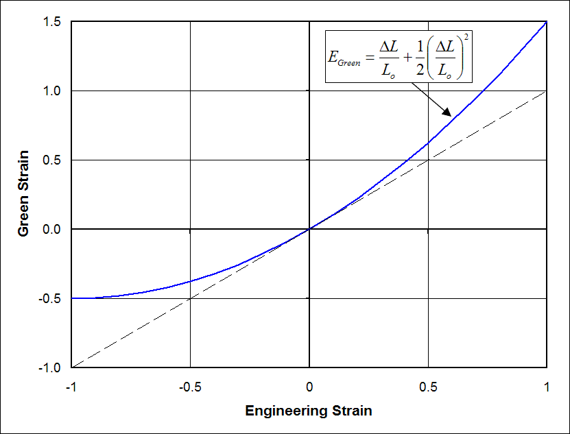
\[ E_{11} = {\Delta L \over L_o} + {1 \over 2} \left( {\Delta L \over L_o} \right)^2 \]
So again, the compromise in a Green strain tensor is the quadratic terms which, while negligible when the strains are small, will cause \({\bf E}\) to be different from engineering strain values when the strains are moderate or large.
Shear Strain

\[ {\partial \, v \over \partial X} = {D \over T} \]
So the engineering and small strain values are
\[ \gamma_{xy} = {\partial \, u \over \partial Y} + {\partial \, v \over \partial X} = {D \over T} \]
The Green strain components are
\[ \begin{eqnarray} E_{xx} & = & {1 \over 2} \left( {\partial \, v \over \partial X} \right)^2 = {1 \over 2} \left( {D \over T} \right)^2 \\ \\ E_{yy} & = & 0 \\ \\ E_{zz} & = & 0 \\ \\ E_{xy} & = & {1 \over 2} {\partial \, v \over \partial X} = {1 \over 2} {D \over T} \\ \\ E_{xz} & = & 0 \\ \\ E_{yz} & = & 0 \end{eqnarray} \]
So the Green strain tensor for this shear case is
\[ {\bf E} = \left[ \matrix{ {1 \over 2} \left( {D \over T} \right)^2 & {1 \over 2} {D \over T} & & 0 \\ \\ {1 \over 2} {D \over T} & 0 & & 0 \\ \\ \\ 0 & 0 & & 0 } \right] \]

\[ \begin{eqnarray} \Delta L \over L_o & = & { \sqrt{T^2 + D^2} - T \over T} \\ \\ & = & \sqrt{1 + \left( {D \over T} \right)^2} - 1 \\ \\ & = & 1 + {1 \over 2} \left( {D \over T} \right)^2 - {1 \over 8} \left( {D \over T} \right)^4 + \;\; ... \;\; - 1 \\ \end{eqnarray} \]
where the last line is a Taylor series expansion of the line above it. This makes it clear that the \(E_{11}\) term is actually the second order effect of stretching of a horizontal line segment due to shear.
An Alternative Derivation
The Green strain is often presented in textbooks in a way that does not highlight its rotational independence, but instead in a way that I feel is more coincidental than physical.Since \({\bf F}\) is defined as
\[ {\bf F} = {\partial \, {\bf x} \over \partial {\bf X}} \]
This means that it can be used to relate an initial undeformed differential length, \({\bf dX}\), to its deformed result, \({\bf dx}\), as follows.
\[ {\bf dx} = {\bf F} \cdot {\bf dX} \qquad \text{because} \qquad {\bf dx} = {\partial \, {\bf x} \over \partial {\bf X}} \cdot {\bf dX} \]
The above relationship is exploited in the following story leading to a derivation of the Green strain tensor. It goes like this...
Since \({\bf dx} = {\bf F} \cdot {\bf dX}\), then
\[ {\bf dx} \cdot {\bf dx} = {\bf F} \cdot {\bf dX} \cdot {\bf F} \cdot {\bf dX} \]
Tensor notation is needed here to figure out how to manipulate this result. So in tensor notation, it is
Which can be recognized as containing a \({\bf F}^T \! \cdot {\bf F}\) term. So this means
\[ \begin{eqnarray} {\bf dx} \cdot {\bf dx} & = & {\bf F} \cdot {\bf dX} \cdot {\bf F} \cdot {\bf dX} \\ \\ & = & {\bf dX} \cdot ( {\bf F}^T \! \cdot {\bf F} ) \cdot {\bf dX} \end{eqnarray} \]
Now subtract \({\bf dX} \cdot {\bf dX}\) from both sides
\[ \begin{eqnarray} {\bf dx} \cdot {\bf dx} - {\bf dX} \cdot {\bf dX} & = & {\bf dX} \cdot ( {\bf F}^T \! \cdot {\bf F} ) \cdot {\bf dX} - {\bf dX} \cdot {\bf dX} \\ \\ & = & {\bf dX} \cdot ( {\bf F}^T \! \cdot {\bf F} ) \cdot {\bf dX} - {\bf dX} \cdot {\bf I} \cdot {\bf dX} \\ \\ & = & {\bf dX} \cdot ( {\bf F}^T \! \cdot {\bf F} - {\bf I}) \cdot {\bf dX} \end{eqnarray} \]
But \({\bf F}^T \! \cdot {\bf F} - {\bf I}\) equals \(2 {\bf E}\). So
\[ {\bf dx} \cdot {\bf dx} - {\bf dX} \cdot {\bf dX} = {\bf dX} \cdot ( 2 {\bf E} ) \cdot {\bf dX} \]
This is used to justify that
\[ E = {ds^2 - dS^2 \over 2 \, dS^2 } \]
where \(ds^2\) is the deformed length squared, and \(dS^2\) is the undeformed length squared.
This is often presented as if it is somehow a better definition of strain than the "boring old" \(\Delta L / L_o\) relationship. But I consider this to only be a coincidence. It is not better at all.
It can be checked by substituting \(L_o\) for \(dS\), and \(L_o + \Delta L\) for \(ds\). It will lead to the now familiar relationship
\[ E \;\; = \;\; {ds^2 - dS^2 \over 2 \, dS^2} \;\; = \;\; {(L_o + \Delta L)^2 - L_o^2 \over 2 \, L_o^2} \;\; = \;\; {\Delta L \over L_o} + {1 \over 2} \left( {\Delta L \over L_o} \right)^2 \]
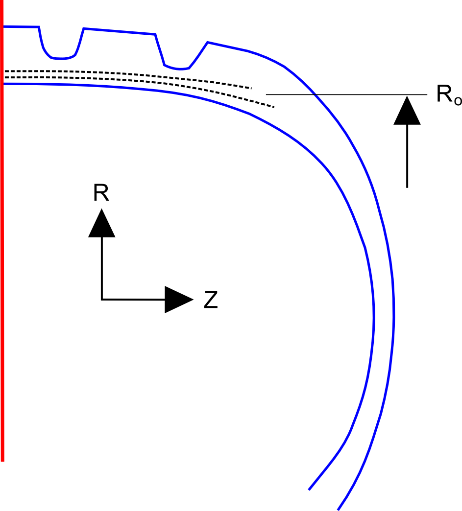
Belt Edge Example
This is an example of computing strains at the belt edge of a tire under high speed axisymmetric centrifugal loading in cylindrical coordinates. The important points to note are...- As always, the first step is to calculate the deformation gradient. The only curve ball is that the partial derivatives in \({\bf F}\) in cylindrical coordinates are more complex than in rectangular coordinates. This is reviewed below.
- However, once \({\bf F}\) is obtained, the remaining steps are identical to those in rectangular coordinates, i.e., \({\bf E} = \frac{1}{2} ({\bf F}^T \! \cdot {\bf F} - {\bf I})\).
\[ {\bf F} \quad = \quad {\bf I} + \nabla {\bf u} \quad = \quad \left[ \matrix { 1 + {\partial \, u_r \over \partial \, R} & {1 \over R} {\partial \, u_r \over \partial \, \theta} - {u_\theta \over R} & {\partial \, u_r \over \partial Z} \\ \\ \\ {\partial \, u_\theta \over \partial \, R} & 1 + {1 \over R} {\partial \, u_\theta \over \partial \, \theta} + {u_r \over R} & {\partial \, u_\theta \over \partial Z} \\ \\ \\ {\partial \, u_z \over \partial \, R} & {1 \over R} {\partial \, u_z \over \partial \, \theta} & 1 + {\partial \, u_z \over \partial Z} } \right] \]
where \(u_r, u_\theta\), and \(u_z\) are the \(R, \theta,\) and \(Z\) components of the displacement vector.
(I've chosen arbitrary values here, in fact.)
\[ \begin{eqnarray} u_r & = & 0.05 R \\ \\ u_\theta & = & -0.2 (R - R_o) \end{eqnarray} \]
Plugging these displacements, at \(R_o\), into the deformation gradient gives
\[ {\bf F} = \left[ \matrix { \;\;\;1.05 & 0 & 0 \\ -0.20 & 1.05 & 0 \\ \;\;0 & 0 & 1 } \right] \]
And the Green strain is
\[ {\bf E} = \left[ \matrix { \;\;\;0.071 & -0.105 & 0 \\ -0.105 & \;\;\;0.051 & 0 \\ \;\;0 & \;\;0 & 0 } \right] \]
Cylindrical coordinates are often nonintuitive, and that seems to apply here as well. There is a substantial amount of circumferential strain, \(E_{\theta \theta}\), in this case even though the displacements are not a function of \(\theta\) at all. This circumferential strain comes from the \(u_r / R\) term in the \(F_{\theta \theta}\) component of \({\bf F}\). The \(u_r / R\) term captures the fact that the deformed circumference, \(2 \pi R_{deformed}\), is different from the initial circumference, \(2 \pi R_o\).
But here's something way more important than the above observation. It is... that once numerical values are calculated from the partial derivatives in \({\bf F}\), the fact that the problem is in cylindrical coordinates goes away. From that point on, the process, interpretation, etc, is identical to that for rectangular coordinates, or any other system for that matter. This is because a strain is a strain is a strain, independent of how you got it (the same is true for stress as well). All the rules for transformations, principal values, hydrostatic and deviatoric components, etc, are the same in rectangular coordinates as in cylindrical coordinates.
Almansi Strain
The Almansi strain tensor, \({\bf e}\), is yet another measure of strain. It always gets covered in discussions of continuum mechanics, but I've never seen it actually used anywhere. So I won't spend much time on it.Its derivation begins similar to the one just above for Green strain. Start with the quantity:
\[ {\bf dx} \cdot {\bf dx} - {\bf dX} \cdot {\bf dX} \]
But this time, substitute the following the identity: \({\bf dX} = {\bf F}^{-1} \! \cdot {\bf dx}\) (Note that \({\bf F}^{-1} = {\partial {\bf X} \over \partial {\bf x}}\))
\[ \begin{eqnarray} {\bf dx} \cdot {\bf dx} - {\bf dX} \cdot {\bf dX} & = & {\bf dx} \cdot {\bf dx} - {\bf F}^{-1} \! \cdot {\bf dx} \cdot {\bf F}^{-1} \! \cdot {\bf dx} \\ \\ & = & {\bf dx} \cdot ({\bf I} - {\bf F}^{-T} \! \cdot {\bf F}^{-1} ) \cdot {\bf dx} \\ \\ & = & {\bf dx} \cdot (2 {\bf e}) \cdot {\bf dx} \end{eqnarray} \]
\[ {\bf e} = \frac{1}{2} ({\bf I} - {\bf F}^{-T} \! \cdot {\bf F}^{-1}) \]
This can also be written as
\[ {\bf e} = \frac{1}{2} ({\bf I} - ({\bf F} \cdot {\bf F}^T)^{-1}) \]
And we already know that \({\bf F} \cdot {\bf F}^T = {\bf V} \cdot {\bf V}^T\). The rotation matrix, \({\bf R}\) has been eliminated from the problem again. So the Almansi strain tensor is independent of rigid body rotations just like the Green strain tensor is.
In terms of the displacement field, it is written as
\[ e_{ij} = {1 \over 2} \left( {\partial \, u_i \over \partial x_j} + {\partial \, u_j \over \partial x_i} - {\partial \, u_k \over \partial x_i} {\partial \, u_k \over \partial x_j} \right) \]
The key here is that the derivatives are with respect to the deformed positions, \({\bf x}\).
Uniaxial Tension with Almansi Strain
\[ u = {x - u \over L_o} (L_F - L_o) \]
and solving for \(u\) gives
\[ u = {x \over L_F} (L_F - L_o) \]
So
\[ {\partial \, u \over \partial \, x} = {\Delta L \over L_F} \]
The \(e_{11}\) component is
\[ e_{11} = {\partial \, u \over \partial x} - {1 \over 2} \left( {\partial \, u \over \partial x} \right)^2 \]
and substituting \(\Delta L / L_F\) gives
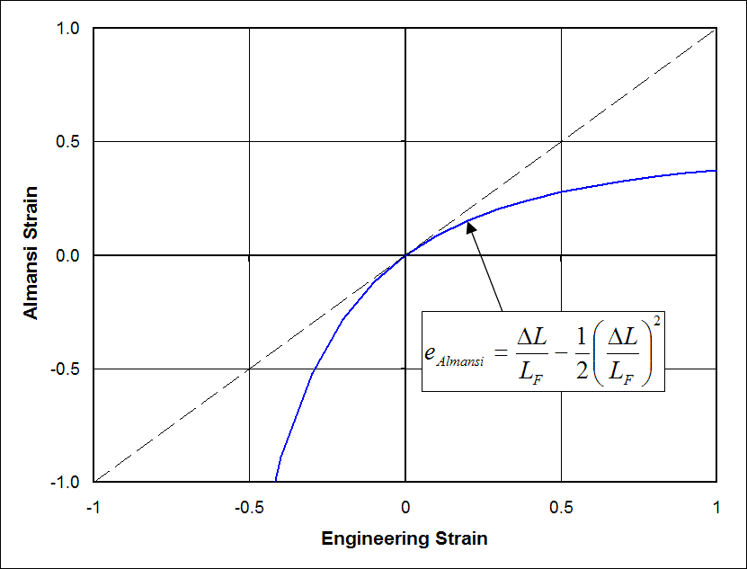
\[ e_{11} = {\Delta L \over L_F} - {1 \over 2} \left( {\Delta L \over L_F} \right)^2 \]
Thank You
Thank you for visiting this webpage. Feel free to email me if you have questions.Also, please consider visiting an advertiser above. Doing so helps to cover website hosting fees.
Bob McGinty
bmcginty@gmail.com
Entire Website - $12.95
For $12.95, you receive two formatted PDFs (the first for 8.5" x 11" pages, the second for tablets) of the entire website.Click here to see a sample page in each of the two formats.
Strain Chapter - $4.99
For $4.99, you receive two formatted PDFs (the first for 8.5" x 11" pages, the second for tablets) of the complete strain chapter.Click here to see a sample page in each of the two formats.
Copyright © 2012 by Bob McGinty