Introduction
This page introduces several definitions of stress. A key discriminator among the different stress tensors is whether they report stress in a material's undeformed, and especially unrotated state, (the reference configuration), or in its deformed and rotated state, (the current configuration).It is interesting that most, perhaps even all, stress definitions can be paired with a corresponding strain tensor. They come in pairs such that the product of the two will give strain energy, hence the name of this page. This does not mean that the corresponding pairs must be used together when performing structural analyses. But they must be when computing strain energy density.
Cauchy Stress (a.k.a. True Stress)
It's been claimed that among the many different strain definitions, no one is necessarily superior to another. They are all just different, each having pros and cons for a given application. However, I don't believe that is the case for stress. For stresses, the Cauchy or True Stress definition appears to be head-and-shoulders more relevant, physical, justified, etc, over other definitions.
Cauchy stress is "force over area in the deformed configuration". So the object has rotated and deformed. And as it has deformed, its cross-sectional area has changed from the undeformed configuration. But it is this rotated and deformed condition that is in final equilibrium, not the reference configuration.
Cauchy stress is represented simply by \(\boldsymbol{\sigma}\). All other stress definitions have some kind of sub or superscripts to indicate what they are.
A very-flimsy diving board is an excellent example of a loading condition that supports this argument. The deformed shape is in equilibrium, not the reference shape. So equilibrium equations involving stresses should be written in terms of the deformed shape, so the Cauchy stress is the natural choice.
Work, Energy, and Power
It is well known that work is the dot-product of force and displacement according to\[ W = \int {\bf F} \cdot {\bf dx} \]
and power is the time-derivative of work, which can be obtained by first taking an infinitesimal amount of work, \( dW = {\bf F} \cdot {\bf dx} \), and dividing through by \(dt\) to obtain
\[ P = {dW \over dt} = {\bf F} \cdot { {\bf dx} \over dt } \]
But \(d{\bf x}/dt\) is simply velocity, \({\bf v}\). So power is
\[ P = {\bf F} \cdot {\bf v} \]
For mechanics calculations, it is often desirable to calculate work and energy in terms of stress and strain rather than force and displacement. Likewise, calculations of power are made in terms of stress and strain-rate instead of force and velocity. The following derivation shows how the quantities are related.
Begin by considering the power generated by forces, both external and internal, acting on an object and moving it at velocity, \({\bf v}\). The external forces will be expressed as traction vectors, \({\bf T}\), acting on the outer surface of the object. The traction vectors must be integrated over the outer surface to obtain force. The internal forces will be represented by \({\bf f}\), having dimensions of force/volume. They arise due to mechanisms such as gravity, accelerations, magnatism, etc. The total force acting on the object will be
The power generated by the forces is computed by simply performing dot-products with the velocity vector, \({\bf v}\).
\[ \text{Power} = \int {\bf T} \cdot {\bf v} \, dA + \int {\bf f} \cdot {\bf v} \, dV \]
Note that \({\bf v}\) need not be constant over the volume (or surface). It can vary due to deformations, rotations, and/or vibrations. Nevertheless, the equation remains correct.
This result can be partitioned into the power associated with motion (involving the velocity vector, \({\bf v}\)), and that associated with deformations (stresses and strains). This is accomplished in a few steps as follows. First, use the traction vector identity, \({\bf T} = \boldsymbol{\sigma} \cdot {\bf n}\), to replace \({\bf T}\) in the equation.
\[ \text{Power} = \int (\boldsymbol{\sigma} \cdot {\bf n}) \cdot {\bf v} \, dA + \int {\bf f} \cdot {\bf v} \, dV \]
Then apply the divergence theorem to the first term containing the surface integral to transform it into a volume integral.
\[ \text{Power} = \int \nabla \cdot (\boldsymbol{\sigma} \cdot {\bf v}) \, dV + \int {\bf f} \cdot {\bf v} \, dV \]
Next, expand the divergence operator to obtain
\[ \text{Power} = \int (\nabla \cdot \boldsymbol{\sigma}) \cdot {\bf v} \, dV + \int \boldsymbol{\sigma} : \nabla{\bf v} \, dV + \int {\bf f} \cdot {\bf v} \, dV \]
The above step is not at all intuitive using matrix notation, but is easily verified with tensor notation. The term, \( \nabla \cdot ( \boldsymbol{\sigma} \cdot {\bf v} ) \) is expressed in tensor notation as \( ( \sigma_{ij} v_i ),_j \). Applying the product rule gives
\[ (\sigma_{ij} v_i ),_j = \sigma_{ij},_j v_i + \sigma_{ij} v_i,_j \]
which is easily interpreted to be
\[ \nabla \cdot (\boldsymbol{\sigma} \cdot {\bf v}) = (\nabla \cdot \boldsymbol{\sigma}) \cdot {\bf v} + \boldsymbol{\sigma} : \nabla{\bf v} \]
The \( \nabla \cdot \boldsymbol{\sigma} \) term is key here because it also appears in the equilibrium equation: \( \nabla \cdot \boldsymbol{\sigma} + {\bf f} = \rho \, {\bf a} \). This makes it possible to replace \( \nabla \cdot \boldsymbol{\sigma} \) with \( ( \rho \, {\bf a} - {\bf f} ) \).
\[ \text{Power} = \int (\rho \, {\bf a} - {\bf f}) \cdot {\bf v} \, dV + \int \boldsymbol{\sigma} : \nabla{\bf v} \, dV + \int {\bf f} \cdot {\bf v} \, dV \]
Expanding the first term out gives
\[ \text{Power} = \int \rho \, {\bf a} \cdot {\bf v} \, dV - \int {\bf f} \cdot {\bf v} \, dV + \int \boldsymbol{\sigma} : \nabla{\bf v} \, dV + \int {\bf f} \cdot {\bf v} \, dV \]
Note that the two \( \int {\bf f} \cdot {\bf v} \, dV \) terms cancel each other, leaving only
\[ \text{Power} = \int \rho \, {\bf a} \cdot {\bf v} \, dV + \int \boldsymbol{\sigma} : \nabla{\bf v} \, dV \]
And the \( \int \rho \, {\bf a} \cdot {\bf v} \, dV \) term is in fact the time derivative of Kinetic Energy: \( \int {1 \over 2} \rho \, ( {\bf v} \cdot {\bf v} ) \, dV \). So it can be written as
\[ \text{Power} = {d \over dt} \left( \int {1 \over 2} \rho \, ( {\bf v} \cdot {\bf v} ) \, dV \right) + \int \boldsymbol{\sigma} : \nabla{\bf v} \, dV \]
Or simply
\[ \text{Power} = {d \over dt} (\text{Kinetic Energy}) + \int \boldsymbol{\sigma} : \nabla{\bf v} \, dV \]
And \( \nabla {\bf v} \) is the velocity gradient, \({\bf L}\). Substitution gives
\[ \text{Power} = {d \over dt} (\text{Kinetic Energy}) + \int \boldsymbol{\sigma} : {\bf L} \, dV \]
And \({\bf L}\) is also equal to \( {\bf D} + {\bf W}\). Substituting and expanding gives
\[ \text{Power} = {d \over dt} (\text{Kinetic Energy}) + \int \boldsymbol{\sigma} : {\bf D} \, dV + \int \boldsymbol{\sigma} : {\bf W} \, dV \]
But \( \boldsymbol{\sigma} : {\bf W} \) is identically zero because \(\boldsymbol{\sigma}\) is symmetric and \({\bf W}\) is antisymmetric. This leaves the final result.
\[ \text{Power} = {d \over dt} (\text{Kinetic Energy}) + \int \boldsymbol{\sigma} : {\bf D} \, dV \]
The total power has now been partitioned into two contributing parts: (i) bulk motion, and (ii) deformations. The bulk motion is represented by kinetic energy, of which the velocity vector, \({\bf v}\), is the key. Deformations are represented by strain energy density, and its rate of change is computed by energetically conjugate pairs of stresses and strain-rates.
We will focus on the deformation component of the total power in order to identify additional pairs of energetically conjugate stresses, strains, and strain-rates. We already have the Cauchy stress and the rate of deformation tensor as our first energetically conjugate pair. This is logical because both are related to the deformed and rotated configuration of an object.
1st Piola Kirchhoff Stress
\[ P = \int \boldsymbol{\sigma} : {\bf D} \, dV \]
But
\[ {\bf D} = {1 \over 2} ({\bf L} + {\bf L}^T) \]
Substitute this into the power calculation.
\[ P = {1 \over 2} \int \boldsymbol{\sigma} : {\bf L} + \boldsymbol{\sigma} : {\bf L}^T \, dV \]
But since \(\boldsymbol{\sigma}\) is symmetric, this reduces to
\[ P = \int \boldsymbol{\sigma} : {\bf L} \, dV \]
and \({\bf L} = \dot {\bf F} \cdot {\bf F}^{-1}\), so substitute
\[ P = \int \boldsymbol{\sigma} : (\dot {\bf F} \cdot {\bf F}^{-1}) \, dV \]
and \(dV = J\,dV_o\). Substitute this to get
\[ P = \int \boldsymbol{\sigma} : (\dot {\bf F} \cdot {\bf F}^{-1}) \, J \, dV_o \]
Once again, converting everything to tensor notation helps to better understand how to regroup components.
\[ P = \int \sigma_{ij} \dot F_{ik} F_{kj}^{-1} \, J \, dV_o \]
Rearrange to get
\[ P = \int \sigma_{ij} F_{kj}^{-1} \dot F_{ik} \, J \, dV_o \]
and take the transpose of the transpose of \(F_{kj}^{-1}\) to get \(F_{jk}^{-T}\).
\[ P = \int J \, \sigma_{ij} F_{jk}^{-T} \dot F_{ik} \, dV_o \]
So this dictates that
\[ P = \int \boldsymbol{\sigma}^{PK1} \! : \dot {\bf F} \, dV_o \]
where
\[ \boldsymbol{\sigma}^{PK1} = J \, \boldsymbol{\sigma} \cdot {\bf F}^{-T} \]
The important result here is that the resulting \(\boldsymbol{\sigma}^{PK1}\) definition is NOT symmetric because, while it is postmultiplied by \({\bf F}^{-T}\), it is not premultiplied by a corresponding \({\bf F}^{-1}\) to make the result symmetric. So this is not a popular stress tensor to use.
2nd Piola Kirchhoff Stress
\[ P = \int \boldsymbol{\sigma} : {\bf D} \, dV \]
This time, use the relationship between \({\bf D}\) and \(\dot {\bf E}\).
\[ {\bf D} = {\bf F}^{-T} \cdot \dot {\bf E} \cdot {\bf F}^{-1} \]
Substitute this into the power calculation.
\[ P = \int \boldsymbol{\sigma} : ({\bf F}^{-T} \cdot \dot {\bf E} \cdot {\bf F}^{-1}) \, dV \]
and \(dV = J\,dV_o\). So substitute to get
\[ P = \int \boldsymbol{\sigma} : ({\bf F}^{-T} \cdot \dot {\bf E} \cdot {\bf F}^{-1}) \, J \, dV_o \]
Once again, converting everything to tensor notation helps to better understand how to regroup components.
\[ P = \int \sigma_{ij} F^{-T}_{im} \dot E_{mn} F^{-1}_{nj} \, J \, dV_o \]
Rearrange to get
\[ P = \int J \, F^{-1}_{mi} \sigma_{ij} F^{-T}_{jn} \dot E_{mn} \, dV_o \]
So this dictates that
\[ P = \int \boldsymbol{\sigma}^{PK2} \! : \dot {\bf E} \, dV_o \]
where
\[ \boldsymbol{\sigma}^{PK2} = J \, {\bf F}^{-1} \! \cdot \boldsymbol{\sigma} \cdot {\bf F}^{-T} \]
\(\boldsymbol{\sigma}^{PK2}\) is symmetric and is a popular stress tensor. It is conjugate to \(\dot {\bf E}\) for power calculations, and conjugate to \({\bf E}\) for energy.
\(\boldsymbol{\sigma}^{PK2}\) is in the reference configuration. Let's plug in the polar decomposition to see this more clearly. Substitute \({\bf U}^{-1} \! \cdot {\bf R}^T\) for \({\bf F}^{-1}\). Recall that \({\bf R}^{-1} = {\bf R}^T\).
And substitute \({\bf R} \cdot {\bf U}^{-1}\) for \({\bf F}^{-T}\). Recall that \({\bf U}\) is symmetric, so \({\bf U}^{-T} = {\bf U}^{-1}\).
This produces
\[ \boldsymbol{\sigma}^{PK2} = J \, {\bf U}^{-1} \! \cdot {\bf R}^T \cdot \boldsymbol{\sigma} \cdot {\bf R} \cdot {\bf U}^{-1} \]
This result is not necessarily useful for calculating \(\boldsymbol{\sigma}^{PK2}\) because it requires a polar decomposition be performed that is otherwise not useful, but it does give insight into the stress definition. For example, the \({\bf R}^T \cdot \boldsymbol{\sigma} \cdot {\bf R}\) term rotates the Cauchy stress from the current configuration back to the reference configuration. This will be demonstrated in examples following the section on engineering stress.
Additional Relationships
Recall the energetically conjugate pairing of the 2nd Piola-Kirchhoff stress and Green strain tensor.\[ P = \int \boldsymbol{\sigma}^{PK2} \! : \dot {\bf E} \, dV_o \]
This immediately means that the following equation is also true.
\[ W''' = \int \boldsymbol{\sigma}^{PK2} \! : d{\bf E} \]
where \(W'''\) is the strain energy per unit volume. (Volume is length3, hence the three apostrophes.)
Engineering Stress
\[ \sigma_{\text{Eng}} = {F_{\text{normal}} \over A_o} \qquad \text{and} \qquad \tau_{\text{Eng}} = {F_{\text{parallel}} \over A_o} \]
But I don't know how to extend these definitions to the case of large rotations.
Stress Examples
Examples here will compare Cauchy stress, 2nd Piola-Kirchhoff stress, and engineering stress. The examples will use incompressible rubber, so \(J = 1\).Simple Tension/Compression of Incompressible Rubber
A rubber test sample is stretched in tension as shown in the figure. It is incompressible, so the volume must remain constant.
\[ L_o \, A_o = L_F \, A_F \]
Rearrange to get
\[ {A_o \over A_F} = {L_F \over L_o} \]
But the ratio of initial to final lengths is related to the engineering strain as follows
\[ {L_F \over L_o} = 1 + \epsilon_{\text{Eng}} \]
So therefore
\[ {A_o \over A_F} = 1 + \epsilon_{\text{Eng}} \]
This relationship will be used to relate the different stress terms. For starters, since in this case, the tensile force is the product of \( ( \sigma \, A_F ) \) and also the product of \( ( \sigma_{\text{Eng}} \, A_o ) \), the two terms can be equated to give
\[ \sigma \, A_F \; = \; \sigma_{\text{Eng}} \, A_o \]
And this can be rearranged to give
\[ { \sigma \over \sigma_{\text{Eng}}} \; = \; { A_o \over A_F } \]
And this can be further manipulated to give
\[ \sigma \; = \; \sigma_{\text{Eng}} ( 1 + \epsilon_{\text{Eng}} ) \]
So when the strains are small, the Cauchy stress and engineering stress are the same for all practical purposes. But as an object is stretched significantly so that its cross-sectional area decreases, the Cauchy stress will become greater than the engineering stress. Likewise, under compression, the opposite case exists. Under compression, the Cauchy stress is less (in absolute value) than the engineering stress.
Relating the Cauchy stress and 2nd Piola-Kirchhoff stress requires computing \({\bf F}\) and then relating the two through
\[ \boldsymbol{\sigma}^{PK2} = J \, {\bf F}^{-1} \! \cdot \boldsymbol{\sigma} \cdot {\bf F}^{-T} \]
For tension/compression of incompressible rubber, the deformation gradient is
\[ {\bf F} = \left[ \matrix{ (1 + \epsilon_{\text{Eng}}) & 0 & 0 \\ \\ 0 & (1 + \epsilon_{\text{Eng}})^{-1/2} & 0 \\ \\ 0 & 0 & (1 + \epsilon_{\text{Eng}})^{-1/2} } \right] \]
Note that its determinant equals one because it is incompressible, \(J = 1\).
Its inverse is
\[ {\bf F}^{-1} = \left[ \matrix{ (1 + \epsilon_{\text{Eng}})^{-1} & 0 & 0 \\ \\ 0 & (1 + \epsilon_{\text{Eng}})^{1/2} & 0 \\ \\ 0 & 0 & (1 + \epsilon_{\text{Eng}})^{1/2} } \right] \]
This leads to
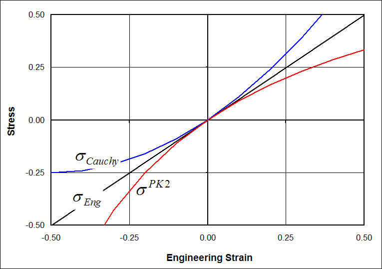
\[ \sigma^{PK2} \; = \; { \sigma \over ( 1 + \epsilon_{\text{Eng}} )^2 } \]
and
\[ \sigma^{PK2} \; = \; { \sigma_{\text{Eng}} \over 1 + \epsilon_{\text{Eng}} } \]
So the deviation of the 2nd Piola-Kirchhoff stress from the engineering stress is just the opposite of the Cauchy stress. When the Cauchy stress is greater than the engineering stress, then \(\sigma^{PK2}\) is less than \(\sigma_{\text{Eng}}\), and vice-versa.
The graph below assumes that \(\sigma_{\text{Eng}} = E \, \epsilon_{\text{Eng}}\) with \(E\) = 1 MPa, roughly the stiffness of natural rubber, at least at smaller strains.
Tension and Rotation of Incompressible Rubber
Recall the example from the page on true strains where the object is stretched and rotated. This time, we will use it to compare stresses in the presence of large rigid body rotations. Engineering stress is not included since it loses meaning in the presence of rotations.
First, the Cauchy stress is simple. The final stress state consists entirely of a normal y-component because the y-direction is the direction of the tensile force. So the final Cauchy stress tensor would look like
\[ \boldsymbol{\sigma} = \left[ \matrix{ 0 & 0 & 0 \\ \\ 0 & F / A & 0 \\ \\ 0 & 0 & 0 } \right] \]
where \(A\) is the final, deformed cross-section of the sample.
The deformation gradient must be determined in order to calculate the 2nd Piola-Kirchhoff stress. The deformation gradient is most easily computed here by taking advantage of the polar decomposition once again. This time
\[ {\bf U} = \left[ \matrix{ (1 + \epsilon_{\text{Eng}}) & 0 & 0 \\ \\ 0 & (1 + \epsilon_{\text{Eng}})^{-1/2} & 0 \\ \\ 0 & 0 & (1 + \epsilon_{\text{Eng}})^{-1/2} } \right] \]
and the rotation matrix is
\[ {\bf R} = \left[ \matrix{ 0 & -1 & \;\;0 \\ \\ 1 & \;\;0 & \;\;0 \\ \\ 0 & \;\;0 & \;\;1 } \right] \]
So the deformation gradient is
\[ \begin{eqnarray} {\bf F} \; = \; {\bf R} \cdot {\bf U} & = & \left[ \matrix{ 0 & -1 & \;\;0 \\ \\ 1 & \;\;0 & \;\;0 \\ \\ 0 & \;\;0 & \;\;1 } \right] \left[ \matrix{ (1 + \epsilon_{\text{Eng}}) & 0 & 0 \\ \\ 0 & (1 + \epsilon_{\text{Eng}})^{-1/2} & 0 \\ \\ 0 & 0 & (1 + \epsilon_{\text{Eng}})^{-1/2} } \right] \\ \\ \\ \\ \\ \\ \\ & = & \left[ \matrix{ 0 & -(1 + \epsilon_{\text{Eng}})^{-1/2} & 0 \\ \\ (1 + \epsilon_{\text{Eng}}) & 0 & 0 \\ \\ 0 & 0 & (1 + \epsilon_{\text{Eng}})^{-1/2} } \right] \end{eqnarray} \]
The inverse of \({\bf F}\) is
\[ {\bf F}^{-1} \; = \; \left[ \matrix{ 0 & (1 + \epsilon_{\text{Eng}})^{-1} & 0 \\ \\ -(1 + \epsilon_{\text{Eng}})^{1/2} & 0 & 0 \\ \\ 0 & 0 & (1 + \epsilon_{\text{Eng}})^{1/2} } \right] \]
The 2nd Piola-Kirchhoff stress is
\[ \boldsymbol{\sigma}^{PK2} = J \, {\bf F}^{-1} \! \cdot \boldsymbol{\sigma} \cdot {\bf F}^{-T} \; = \; \left[ \matrix{ {F / A \over (1 + \epsilon_{\text{Eng}})^2} & 0 & \;\;\;\;\;0 \\ \\ 0 & 0 & \;\;\;\;\;0 \\ \\ 0 & 0 & \;\;\;\;\;0 } \right] \]
The 2nd Piola-Kirchhoff stress has a nonzero component in the normal-x location because the force acts on the object in a direction that was initially in the x-direction.
The term amounts to being \(\sigma / (1 + \epsilon_{\text{Eng}})^2\), but could also be written as \(\sigma_{\text{Eng}} / (1 + \epsilon_{\text{Eng}})\) for this simple tension case.
\(\boldsymbol{\sigma}^{\text{PK2}}\) is less than \(\boldsymbol{\sigma}\) while \(\dot {\bf E}\) is greater than \({\bf D}\) by just the right amount such that \(\boldsymbol{\sigma}^{\text{PK2}} : \dot {\bf E}\) is exactly equal to \(\boldsymbol{\sigma} : {\bf D}\). Each pair is energetically conjugate.
A Note Concerning Linear Elasticity
We've talked about Hooke's Law relating stress and strain in the section on tensor notation. Recall that\[ \boldsymbol{\epsilon} = {1 \over E} \left[ (1 + \nu) \boldsymbol{\sigma} - \nu \; {\bf I} \; \text{tr}(\boldsymbol{\sigma}) \right] \]
But we glossed over the issue of which stress and strain tensors should be used in the equation.
The answer is deceptively simple... in most cases. This is because linear elasticity only applies to very small strains, typically <1%. And now we've seen that all stress definitions are equivalent, as well all strain definitions, when the strains are small. So it doesn't really matter, in fact.
However, there is a gotcha. It is, as usual, rotations. In the presence of large rotations, the proper pairing of stress and strain is critical. Recall the earlier example of the object rotating while being stretched.
Of course, the level of stretching here is too large to be considered linear elastic. But it serves the purpose for this discussion of rotations.
It is easy, and perfectly correct, to write the equation in terms of \(\boldsymbol{\sigma}^{\text{PK2}}\) and \({\bf E}\) as
\[ {\bf E} = {1 \over E} \left[ (1 + \nu) \boldsymbol{\sigma}^{\text{PK2}} - \nu \; {\bf I} \; \text{tr}(\boldsymbol{\sigma}^{\text{PK2}}) \right] \]
This will work no matter the level or rotation. Just be careful that \({\bf E}\) is strain and \(E\) is the elastic modulus.
One could equally well write it in rate form as
\[ \dot {\bf E} = {1 \over E} \left[ (1 + \nu) \dot{\boldsymbol{\sigma}}^{\text{PK2}} - \nu \; {\bf I} \; \text{tr}( \dot{\boldsymbol{\sigma}}^{\text{PK2}}) \right] \]
Likewise, one could write Hooke's Law in terms of \(\boldsymbol{\sigma}\) and \(\boldsymbol{\epsilon}_{\text{True}}\) (as long as \(\boldsymbol{\epsilon}_{\text{True}}\) is computed in the current orientation).
\[ \boldsymbol{\epsilon}_{\text{True}} = {1 \over E} \left[ (1 + \nu) \boldsymbol{\sigma} - \nu \; {\bf I} \; \text{tr}(\boldsymbol{\sigma}) \right] \]
But guess what. The one thing that cannot be done (at least correctly) is to write it in terms of \(\dot{\boldsymbol{\sigma}}\) and \(\dot{\boldsymbol{\epsilon}}_{\text{True}}\) (\(={\bf D}\)).
To see this, consider a slight alternative of the above figure. Think of the object as first being stretched in the x-direction, and then being held at a constant length. This produces a stress in the x-direction that is constant while the object is held at constant length. And note that \(\dot{\boldsymbol{\epsilon}}_{\text{True}}\) (\(={\bf D}\)) is zero as a result.
So far, so good. But the problem arises when the now-stretched object starts to rotate from a horizontal to vertical orientation. The Cauchy stress starts in the x-normal component, but transitions to the y-normal component as the object rotates. So there are definitely non-zero components in \(\dot{\boldsymbol{\sigma}}\) because the components of \(\boldsymbol{\sigma}\) are changing with time. But there is no \({\bf D}\) at all because the object is not stretching; it is only rotating.
So here we have a major problem in that \(\dot{\boldsymbol{\sigma}}\) is not zero while \({\bf D}\) is zero. This leads to the issue of corotational derivatives, which address this disparity. We will cover them in more detail a little later.