Stress Transformations

Introduction

As with strain, transformations of stress tensors follow the same rules of pre and post multiplying by a transformation or rotation matrix regardless of which stress or strain definition one is using. The only difference is that the full shear values, \(\tau_{ij}\), are used in stress tensors and their transformations, not the half shear values, \(\gamma/2\), used in strain tensors.

This page will cover coordinate transformations and rotations in 2-D and 3-D.

2-D Coordinate Transforms of Stress

Coordinate transforms represent rotations of the coordinate system while the object is held constant. The common application of coordinate transforms is to rotate the coordinate system to find the principal directions of the stress tensor. The governing equations are derived by summing forces on differential objects. The sketch here demonstrates this for the (relatively) simple 2-D case.

Summing forces in the x and y directions gives

\[ \sigma_{xx} \, A \, \cos \theta + \tau_{xy} \, A \, \sin \theta = \sigma' \, A \, \cos \theta - \tau' \, A \, \sin \theta \] \[ \tau_{xy} \, A \, \cos \theta + \sigma_{yy} \, A \, \sin \theta = \sigma' \, A \, \sin \theta + \tau' \, A \, \cos \theta \]
The area, \(A\), cancels out of both sides leaving

\[ \begin{eqnarray} \sigma_{xx} \, \cos \theta + \tau_{xy} \, \sin \theta & = & \sigma' \, \cos \theta - \tau' \, \sin \theta \\ \\ \tau_{xy} \, \cos \theta + \sigma_{yy} \, \sin \theta & = & \sigma' \, \sin \theta + \tau' \, \cos \theta \end{eqnarray} \]
This represents two simultaneous equations with two unknowns, \(\sigma'\) and \(\tau'\). Solving the equations gives the well-known 2-D stress transformation equations.

\[ \begin{eqnarray} \sigma' & = & \sigma_{xx} \, \cos^2 \theta + \sigma_{yy} \, \sin^2 \theta + 2 \, \tau_{xy} \sin \theta \cos \theta \\ \\ \tau' & = & (\sigma_{yy} - \sigma_{xx}) \sin \theta \cos \theta + \tau_{xy} ( \cos^2 \theta - \sin^2 \theta ) \end{eqnarray} \]
This gives the normal and shear stresses on any face and is, in fact, the exact same result as obtained on the earlier page on traction vectors, except this is 2-D, of course. The complete transformed 2-D stress state is obtained by evaluating these two equations, plus one additional equation for normal stress at \(\theta + 90^\circ\).

\[ \begin{eqnarray} \sigma'\!_{xx} & = & \sigma_{xx} \, \cos^2 \theta + \sigma_{yy} \, \sin^2 \theta + 2 \, \tau_{xy} \sin \theta \cos \theta \\ \\ \sigma'\!_{yy} & = & \sigma_{xx} \, \sin^2 \theta + \sigma_{yy} \, \cos^2 \theta - 2 \, \tau_{xy} \sin \theta \cos \theta \\ \\ \tau'\!_{xy} & = & (\sigma_{yy} - \sigma_{xx}) \sin \theta \cos \theta + \tau_{xy} (\cos^2 \theta - \sin^2 \theta) \end{eqnarray} \]
The complete set of transformation equations can be summarized in matrix form as

\[ \left[ \matrix{\sigma'_{xx} & \tau'_{xy} \\ \tau'_{xy} & \sigma'_{yy} } \right] = \left[ \matrix{\;\;\; \cos \theta & \sin \theta \\ -\sin \theta & \cos \theta } \right] \left[ \matrix{\sigma_{xx} & \tau_{xy} \\ \tau_{xy} & \sigma_{yy} } \right] \left[ \matrix{\cos \theta & -\sin \theta \\ \sin \theta & \;\;\; \cos \theta } \right] \]
The leading and trailing matrices are the familiar \({\bf Q}\) matrix and its transpose. The complete set of equations can be written simply as

\[ \boldsymbol{\sigma'} = {\bf Q} \cdot \boldsymbol{\sigma} \cdot {\bf Q}^T \]

2-D Stress Transform Example

If the stress tensor in a reference coordinate system is \( \left[ \matrix{1 & 2 \\ 2 & 3 } \right] \), then in a coordinate system rotated 50°, it would be written as

\[ \begin{eqnarray} \left[ \matrix{\sigma'_{xx} & \sigma'_{xy} \\ \sigma'_{xy} & \sigma'_{yy} } \right] & = & \left[ \matrix{\;\;\; \cos 50^\circ & \sin 50^\circ \\ -\sin 50^\circ & \cos 50^\circ } \right] \left[ \matrix{1 & 2 \\ 2 & 3 } \right] \left[ \matrix{\cos 50^\circ & -\sin 50^\circ \\ \sin 50^\circ & \;\;\; \cos 50^\circ } \right] \\ \\ & = & \left[ \matrix{4.143 & \;\;\; 0.638 \\ 0.638 & -0.143 } \right] \end{eqnarray} \]
The stress state has not changed at all. Only the values of the individual components are different because the orientations of the coordinate systems are different.

Tensor Notation

The coordinate transform is written in tensor notation as

\[ \sigma'_{mn} = \lambda_{mi} \lambda_{nj} \sigma_{ij} \]
As usual, tensor notation provides extra insight into the process. This time, the insight comes from the subscripts on the lambdas. Each lambda effectively pairs up a subscript on \(\boldsymbol{\sigma'}\) with one on \(\boldsymbol{\sigma}\). This is true regardless of the rank of the tensor.

3-D Coordinate Transforms

Once again, the rules don't change, only the particulars do.

\[ \boldsymbol{\sigma'} = {\bf Q} \cdot \boldsymbol{\sigma} \cdot {\bf Q}^T \qquad \qquad \qquad \qquad \sigma'_{mn} = \lambda_{mi} \lambda_{nj} \sigma_{ij} \qquad \qquad \qquad \qquad \lambda_{ij} = \cos(x'_i,x_j) \]
Writing the matrices out explicitly gives

\[ \left[ \matrix{\sigma'\!_{xx} & \sigma'\!_{xy} & \sigma'\!_{xz} \\ \sigma'\!_{xy} & \sigma'\!_{yy} & \sigma'\!_{yz} \\ \sigma'\!_{xz} & \sigma'\!_{yz} & \sigma'\!_{zz} } \right] = \left[ \matrix { Q_{11} & Q_{12} & Q_{13} \\ Q_{21} & Q_{22} & Q_{23} \\ Q_{31} & Q_{32} & Q_{33} } \right] \left[ \matrix{\sigma_{xx} & \sigma_{xy} & \sigma_{xz} \\ \sigma_{xy} & \sigma_{yy} & \sigma_{yz} \\ \sigma_{xz} & \sigma_{yz} & \sigma_{zz} } \right] \left[ \matrix { Q_{11} & Q_{21} & Q_{31} \\ Q_{12} & Q_{22} & Q_{32} \\ Q_{13} & Q_{23} & Q_{33} } \right] \]
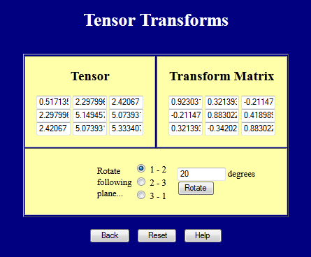
This webpage performs coordinate transforms on 3-D tensors. Try it out.

Rotations

Rotations are the process in which the object rotates while the coordinate system remains fixed. The rotation matrix, \({\bf R}\), is usually computed from a polar decomposition. The rotated stress tensor is calculated as

\[ \boldsymbol{\sigma'} = {\bf R} \cdot \boldsymbol{\sigma} \cdot {\bf R}^T \]
which looks like this in 3-D.

\[ \left[ \matrix{\sigma'\!_{xx} & \sigma'\!_{xy} & \sigma'\!_{xz} \\ \sigma'\!_{xy} & \sigma'\!_{yy} & \sigma'\!_{yz} \\ \sigma'\!_{xz} & \sigma'\!_{yz} & \sigma'\!_{zz} } \right] = \left[ \matrix { R_{11} & R_{12} & R_{13} \\ R_{21} & R_{22} & R_{23} \\ R_{31} & R_{32} & R_{33} } \right] \left[ \matrix{\sigma_{xx} & \sigma_{xy} & \sigma_{xz} \\ \sigma_{xy} & \sigma_{yy} & \sigma_{yz} \\ \sigma_{xz} & \sigma_{yz} & \sigma_{zz} } \right] \left[ \matrix { R_{11} & R_{21} & R_{31} \\ R_{12} & R_{22} & R_{32} \\ R_{13} & R_{23} & R_{33} } \right] \]
In 2-D, the rotation matrix is the transpose of the coordinate transformation matrix.

\[ {\bf R} = \left[ \matrix{\cos \theta & -\sin \theta \\ \sin \theta & \;\;\; \cos \theta } \right] \qquad \qquad {\bf Q} = \left[ \matrix{\;\;\; \cos \theta & \sin \theta \\ -\sin \theta & \cos \theta } \right] \]

So for a 2-D rigid body rotation of \(\theta\) degrees, the equations are

\[ \begin{eqnarray} \sigma'\!_{xx} & = & \sigma_{xx} \, \cos^2 \theta + \sigma_{yy} \, \sin^2 \theta - 2 \, \tau_{xy} \sin \theta \cos \theta \\ \\ \sigma'\!_{yy} & = & \sigma_{xx} \, \sin^2 \theta + \sigma_{yy} \, \cos^2 \theta + 2 \, \tau_{xy} \sin \theta \cos \theta \\ \\ \tau'\!_{xy} & = & (\sigma_{xx} - \sigma_{yy}) \sin \theta \cos \theta + \tau_{xy} (\cos^2 \theta - \sin^2 \theta) \end{eqnarray} \]

2-D Stress Rotation Example

Take the coordinate transformation example from above and this time apply a rigid body rotation of 50° instead of a coordinate transformation.

If the stress tensor in a reference coordinate system is \( \left[ \matrix{1 & 2 \\ 2 & 3 } \right] \), then after rotating 50°, it would be

\[ \begin{eqnarray} \left[ \matrix{\sigma'\!_{xx} & \sigma'\!_{xy} \\ \sigma'\!_{xy} & \sigma'\!_{yy} } \right] & = & \left[ \matrix{\cos 50^\circ & -\sin 50^\circ \\ \sin 50^\circ & \;\;\; \cos 50^\circ } \right] \left[ \matrix{1 & 2 \\ 2 & 3 } \right] \left[ \matrix{\;\;\; \cos 50^\circ & \sin 50^\circ \\ -\sin 50^\circ & \cos 50^\circ } \right] \\ \\ & = & \left[ \matrix{\;\;\; 0.204 & -1.332 \\ -1.332 & \;\;\; 3.796 } \right] \end{eqnarray} \]
The stress state has not changed at all. Only the values of the individual components are different because the object has rotated relative to the global coordinate system.

Rotating and Transforming Back

Start with the above rotation equation.

\[ \boldsymbol{\sigma'} = {\bf R} \cdot \boldsymbol{\sigma} \cdot {\bf R}^T \]
Premultiply both sides by \({\bf R}'\) and postmultiply both sides by \({\bf R}\).

\[ {\bf R}^T \! \cdot \boldsymbol{\sigma'} \cdot {\bf R} = {\bf R}^T \! \cdot {\bf R} \cdot \boldsymbol{\sigma} \cdot {\bf R}^T \cdot {\bf R} \]
The \({\bf R}\) and \({\bf R}^T\) matrices cancel out (because \({\bf R}^T \! = {\bf R}^{-1}\)) leaving

\[ {\bf R}^T \cdot \boldsymbol{\sigma'} \cdot {\bf R} = \boldsymbol{\sigma} \]
The process of transforming a coordinate system back to its original orientation is exactly the same. The equation to do this is

\[ \boldsymbol{\sigma} = {\bf Q}^T \! \cdot \boldsymbol{\sigma'} \cdot {\bf Q} \]