Hydrostatic & Deviatoric Strains

Introduction

This page introduces hydrostatic and deviatoric strains. The two are subsets of any given strain tensor, which, when added together, give the original strain tensor back. The hydrostatic strain is closely related to volume change, while the deviatoric strain is related to deformation at constant volume.

Hydrostatic Strain

Hydrostatic strain is simply the average of the three normal strains of any strain tensor.

\[ \epsilon_{Hyd} = {\epsilon_{11} + \epsilon_{22} + \epsilon_{33} \over 3} \]
And there are many alternative ways to write this.

\[ \epsilon_{Hyd} \; = \; {1 \over 3} \text{tr}(\boldsymbol{\epsilon}) \; = \; {1 \over 3} I_1 \; = \; {1 \over 3} \epsilon_{kk} \]
It is a scalar quantity, although it is regularly used in tensor form as

\[ \boldsymbol{\epsilon_{Hyd}} = \left[ \matrix{\epsilon_{Hyd} & 0 & 0 \\ 0 & \epsilon_{Hyd} & 0 \\ 0 & 0 & \epsilon_{Hyd} } \right] \]

Hydrostatic Strain Example

Hydrostatic Strains and Coordinate Transformations

This could not be simpler. Hydrostatic strains do not change under coordinate transformations. This is easily accepted in light of the fact that \(\epsilon_{Hyd}\) is a function of \(I_1\). Also

\[ \boldsymbol{\epsilon}_{Hyd} = \left[ \matrix{\epsilon_{Hyd} & 0 & 0 \\ 0 & \epsilon_{Hyd} & 0 \\ 0 & 0 & \epsilon_{Hyd} } \right] \]
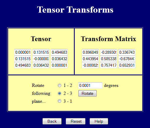
contains equal amounts of strain in all three directions. In fact, it contains equal strain in all directions. And since the tensor does not change under any transformation, this means that no shear strains ever arise, so every direction is a principal direction with \(\epsilon_{Hyd}\) strain.

Hydrostatic and Volumetric Strains

Hydrostatic strain is closely related to volume change in an object, especially when the strains are small. It is less-so at large strains. And this time, it really is an issue of large-vs-small strain, not large-vs-small rotations.

Consider the object in the sketch here. We will look at its volume change. Its initial volume is \(V_o = W_o D_o H_o\) and its final volume is \(V_F = W_F D_F H_F\).

It can be thought of as being aligned with the principal strain tensor and this is why there are no shears. Let the principal strains be defined as

\[ \epsilon_i = {\Delta L \over L_o} \]
where \(L\) can be \(W\), \(D\), or \(H\). So

\[ \begin{eqnarray} W_F & = & W_o ( 1 + \epsilon_1) \\ \\ D_F & = & D_o ( 1 + \epsilon_2) \\ \\ H_F & = & H_o ( 1 + \epsilon_3) \\ \end{eqnarray} \]
Now look at the ratio of \(V_F\) to \(V_o\).

\[ {V_F \over V_o} = {W_F D_F H_F \over W_o D_o H_o } \]
Substituting the strain equations gives

\[ {V_F \over V_o} = ( 1 + \epsilon_1) ( 1 + \epsilon_2) ( 1 + \epsilon_3) \]
and expanding this out gives

\[ {V_F \over V_o} = 1 + \epsilon_1 + \epsilon_2 + \epsilon_3 + \epsilon_1 \epsilon_2 + \epsilon_2 \epsilon_3 + \epsilon_3 \epsilon_1 + \epsilon_1 \epsilon_2 \epsilon_3 \]
Now, if the strains are small, then the products will be negligible and can be ignored. This leaves

\[ {V_F \over V_o} \approx 1 + \epsilon_1 + \epsilon_2 + \epsilon_3 \qquad \text{(small strains)} \]
which can be manipulated to give

\[ {V_F \over V_o} \approx 1 + 3 \left( {\epsilon_1 + \epsilon_2 + \epsilon_3 \over 3} \right) = 1 + 3 \epsilon_{Hyd} \]
So \(\epsilon_{Hyd}\) is directly related to volume change when the strains are small. Also, volumetric strain can be defined as

\[ \epsilon_{Vol} = {\Delta V \over V_o} \]
and this leads to

\[ \epsilon_{Vol} = \epsilon_1 + \epsilon_2 + \epsilon_3 \qquad \text{(small strains)} \]
Note that the sum of principal strains here is an invariant, so the sum can in fact be made at anytime, not just when the normal strains are principals.

But this is just

\[ \epsilon_{Vol} = 3 \, \epsilon_{Hyd} \]

Volumetric Strain Under Large Strains

Now return to the earlier equation that gave the exact ratio between the initial and final volumes.

\[ {V_F \over V_o} = ( 1 + \epsilon_1) ( 1 + \epsilon_2) ( 1 + \epsilon_3) \]

This equation is exact for all strains as long as the principal strains are defined as \(\Delta L / L_o\). The equation is in fact the determinant of \({\bf I} + \boldsymbol{\epsilon}_P\). But \({\bf I} + \boldsymbol{\epsilon}_P\) is just \({\bf U}\) in the principal orientation, so it is also the determinant of \({\bf U}\). And this means that \(\text{det}({\bf U})\) is \(V_F / V_o\).

Recall that computing \({\bf U}\) is pretty difficult, so one might initially think that there is no easy way to find \(V_F / V_o\). But one would be wrong! It turns out that \(\text{det}({\bf U})\) is exactly equal to \(\text{det}({\bf F})\) because \({\bf R}\) does not alter the determinant. So

\[ {V_F \over V_o} = \text{det}({\bf F}) \qquad \text{(all strains, always)} \]
This is such an important result that \(\text{det}({\bf F})\) is given a special symbol, \(J\), and a special name, the Jacobian.

Hydrostatic Strain in Incompressible Materials

A confusing aspect of hydrostatic strain is that it can be nonzero in incompressible materials. This comes from the fact that hydrostatic strain is in fact a mathematical construct more than a direct physical measure of volume and its change. After all, it is the determinant of the deformation gradient that is the true measure of volume change, and hydrostatic strain is only a convenient approximation of that when the strains are small.

At large strains, hydrostatic strain loses its link to volume because it is no longer an approximation of its change. It is reduced to a mere mathematical property of a strain tensor. One can get a feel for this using the two examples below.

Hydrostatic Strain Under Tension/Compression

For simple tension and compression of an incompressible material, the principal strains must satisfy

\[ {V_F \over V_o} = ( 1 + \epsilon_1) ( 1 + \epsilon_2) ( 1 + \epsilon_3) = 1 \]
Select "1" as the tension/compression direction and call that strain \(\epsilon_{Eng}\). The other two strains must be equal. Call both of them, \(\epsilon_{other}\). This gives

\[ ( 1 + \epsilon_{Eng}) ( 1 + \epsilon_{other})^2 = 1 \]
Solving for \(\epsilon_{other}\) gives

\[ \epsilon_{other} = \sqrt{1 \over 1 + \epsilon_{Eng}} - 1 \]
and combining two of these with one \(\epsilon_{Eng}\) to get \(\epsilon_{Hyd}\) gives

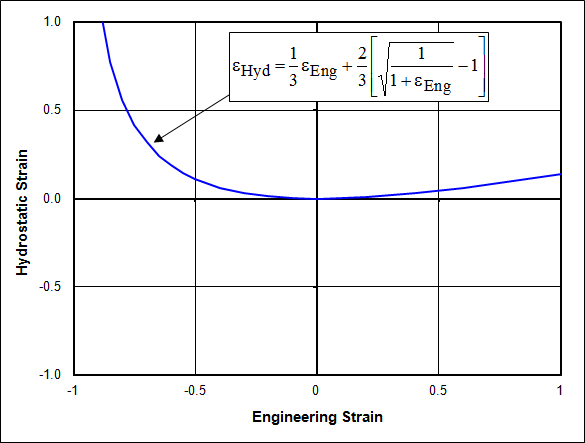
\[ \epsilon_{Hyd} = {1 \over 3} \epsilon_{Eng} + {2 \over 3} \left[ \sqrt{1 \over 1 + \epsilon_{Eng}} - 1 \right] \]
The function is graphed below. You can see that \(\epsilon_{Hyd}\) is very close to zero at small strains, correctly reflecting that the volume does not change. But at large strains, \(\epsilon_{Hyd}\) drifts into positive territory, even though the volume is not changing.

Hydrostatic Strain Under Shear

The principal strains for pure shear are \(\epsilon_1 = \gamma / 2\) and \(\epsilon_2 = -\gamma / 2\). So the strain tensor looks like

\[ \boldsymbol{\epsilon}_P = \left[ \matrix{ \gamma/2 & 0 & 0 \\ 0 & -\gamma/2 & 0 \\ 0 & 0 & \epsilon_3 } \right] \] And the ratio of initial to final volume is

\[ {V_F \over V_o} = ( 1 + \gamma / 2) ( 1 - \gamma / 2) ( 1 + \epsilon_3) = 1 \]
Solve for \(\epsilon_3\) to get

\[ \epsilon_3 = {1 \over 1 - \left( { \gamma \over 2} \right)^2 } - 1 \]
And the hydrostatic strain is

\[ \epsilon_{Hyd} = {1 \over 3} \left[ {1 \over 1 - \left( { \gamma \over 2} \right)^2 } - 1 \right] \]

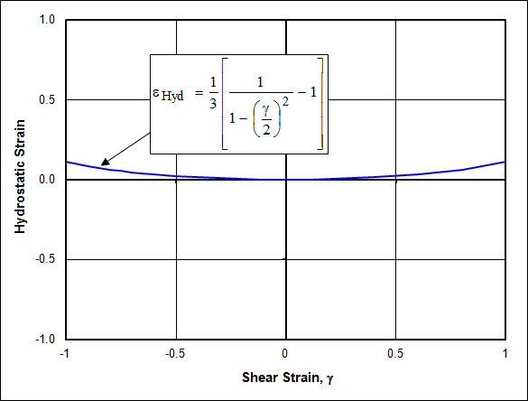
The deviation from zero is much less severe in this case than for tension and compression. Nevertheless, it is still present because hydrostatic strain is only an approximation of volume change, not an exact measure.

Deviatoric Strain

Deviatoric strain is what's left after subtracting out the hydrostatic strain. If the strains are small, then it is all the deformations that cause a shape change without changing the volume.

The deviatoric strain will be represented by \(\boldsymbol{\epsilon}'\), or \({\bf E}'\), or \({\bf e}'\) depending on what the starting strain tensor is. For example

\[ \boldsymbol{\epsilon}' = \boldsymbol{\epsilon} - \boldsymbol{\epsilon}_{Hyd} \]
In tensor notation, it is written as

\[ \epsilon'\!_{ij} = \epsilon_{ij} - {1 \over 3} \delta_{ij} \epsilon_{kk} \]

Deviatoric Strain Example

Given the following Green strain tensor

\[ {\bf E} = \left[ \matrix{ 0.50 & \;\;\; 0.30 & \;\;\;0.20 \\ 0.30 & -0.20 & -0.10 \\ 0.20 & -0.10 & \;\;\;0.10 } \right] \]
The hydrostatic strain is

\[ E_{Hyd} \, = \, {0.50 + (-0.20) + 0.10 \over 3} \, = \, 0.133 \]
which can be written as

\[ {\bf E}_{Hyd} = \left[ \matrix{ 0.133 & 0 & 0 \\ 0 & 0.133 & 0 \\ 0 & 0 & 0.133 } \right] \]
Subtracting the hydrostatic strain tensor from the total strain gives

\[ {\bf E}' = \left[ \matrix{ 0.50 & \;\;\; 0.30 & \;\;\;0.20 \\ 0.30 & -0.20 & -0.10 \\ 0.20 & -0.10 & \;\;\;0.10 } \right] - \left[ \matrix{ 0.133 & 0 & 0 \\ 0 & 0.133 & 0 \\ 0 & 0 & 0.133 } \right] = \left[ \matrix{ 0.367 & \;\;\; 0.300 & \;\;\;0.200 \\ 0.300 & -0.333 & -0.100 \\ 0.200 & -0.100 & -0.033 } \right] \]
Note that the result is traceless. Its first invariant equals zero. Or put another way, the hydrostatic strain of a deviatoric strain tensor is zero.

An interesting aspect of a traceless tensor is that it can be formed entirely from shear components. For example, a coordinate system transformation can be found to express the deviatoric strain tensor in the above example as shear strain exclusively. In the screenshot here, the above deviatoric strain tensor was input into the webpage, and then the coordinate system was rotated until the following strain tensor was obtained.

Once again, note that just because all the normal strains are zero, this does not mean that the strain tensor represents a constant volume deformation. A simple example demonstrating this is the case of pure shear. Starting from

\[ \boldsymbol{\epsilon} = \left[ \matrix{ 0 & \gamma / 2 & 0 \\ \gamma / 2 & 0 & 0 \\ 0 & 0 & 0 } \right] \]
The principal strain tensor is

\[ \boldsymbol{\epsilon}_P = \left[ \matrix{ \gamma / 2 & \;0 & 0 \\ 0 & -\gamma / 2 & 0 \\ 0 & \;0 & 0 } \right] \]
And so the determinant of \({\bf I} + \boldsymbol{\epsilon}_P\) equals

\[ {V_F \over V_o} = ( 1 + \gamma / 2) ( 1 - \gamma / 2) = 1 - (\gamma / 2)^2 \]
which decreases with increasing shear strain.

Constant Volume Deformation

Let's close with an example that is in fact a constant volume deformation - the case of simple shear.

\[ \gamma = {D \over T} \]
For this case, the deformation gradient is

\[ {\bf F} = \left[ \matrix{ 1 & 0 & 0 \\ \gamma & 1 & 0 \\ 0 & 0 & 1 } \right] \]
and its determinant is indeed 1 regardless of the value of \(\gamma\), so it truly is a constant volume deformation. (Recall that the determinant of \({\bf F}\) always gives the exact ratio of \(V_F / V_o\).)

The Green strain tensor for this case is

\[ {\bf E} = \left[ \matrix{ \gamma^2 / 2 & \gamma / 2 & 0 \\ \gamma / 2 & 0 & 0 \\ 0 & 0 & 0 } \right] \]
So the hyrdrostatic strain tensor is

\[ {\bf E}_{Hyd} = \left[ \matrix{ \gamma^2 / 6 & 0 & 0 \\ 0 & \gamma^2 / 6 & 0 \\ 0 & 0 & \gamma^2 / 6 } \right] \]
And the deviatoric strain tensor is

\[ {\bf E}' = \left[ \matrix{ \gamma^2 / 3 & \gamma / 2 & 0 \\ \gamma / 2 & -\gamma^2 / 6 & 0 \\ 0 & 0 & -\gamma^2 / 6 } \right] \]