Introduction
Mooney-Rivlin models are popular for modeling the large strain nonlinear behavior of incompressible materials, i.e., rubber. It's important to understand that Mooney-Rivlin models do not give any special insight into material behavior. They are merely curve-fits of various polynomials to test data. The numerical values of coefficients resulting from the curve-fits are entered into FEA programs for use in mechanical analyses. The FEA program knows how stiff the rubber is based on the values of the coefficients.Keep in mind that auto-summation of duplicated subscripts will not apply to the equations on this page. Hopefully, the reasons for this will be obvious!
Strain Energy
\[ \boldsymbol{\sigma}^\text{PK2} = \rho_o \, {\partial \Psi \over \partial {\bf E}^\text{el} } \]
The Helmholtz free energy contains thermal energy and mechanical strain energy. But in most every discussion of Mooney-Rivlin coefficients, the thermal part is neglected, leaving only the mechanical part, \(W\). (Actually, \(W\) is declared to represent \(\rho_o \Psi\), not just \(\Psi\)). Second, since all of the deformation of a hyperelastic material is elastic by definition, it is sufficient to write \({\bf E}^\text{el}\) simply as \({\bf E}\). This gives
\[ \boldsymbol{\sigma}^\text{PK2} = {\partial W \over \partial {\bf E} } \]
But there is a challenge with this general approach. It is the determination of off-diagonal (shear) terms. As with the shear terms in Hooke's Law, they are not independent of the normal terms, but must be consistent with coordinate transformations that transform normal components into shears and vice-versa. And as with Hooke's Law, the resolution is to define the material behavior for the principal values and rely on coordinate transformations to give the appropriate corresponding behavior of the shear terms.
\[ \sigma_i^\text{PK2} = {\partial W \over \partial E_i } \]
But alas, even this is not quite what is done in Mooney-Rivlin models. Instead, derivatives are taken with respect to stretch ratios, \(\lambda\), which are the ratios of initial and final lengths in the principal directions, \((L_F / L_o)\). So the stretch ratio is "one plus engineering strain," \(\lambda = 1 + \epsilon_{Eng}\), and therefore \(\lambda - 1 = \epsilon_{Eng} = \Delta L \, / L_o\).
We can get there using the chain rule.
\[ \sigma_i^\text{PK2} = {\partial W \over \partial E_i } = {\partial W \over \partial \lambda_i } {\partial \lambda_i \over \partial E_i} \]
We just need an equation relating \(E_i\) to \(\lambda_i\). Recall that a principal Green strain equals
\[ E_i = {\Delta L_i \over L_o} + {1 \over 2} \left( {\Delta L_i \over L_o} \right)^2 \]
And insert the relationship \(\lambda_i - 1 = \Delta L_i / L_o\) to get
\[ E_i = (\lambda_i - 1) + {1 \over 2} (\lambda_i - 1)^2 \]
So \(\partial E_i / \partial \lambda_i = \lambda_i\) and therefore
\[ {\partial \lambda_i \over \partial E_i } = {1 \over \lambda_i} \]
Substituting this into the equation containing \(\sigma^\text{PK2}\) and \(W\) gives
\[ \sigma_i^\text{PK2} = {1 \over \lambda_i} {\partial W \over \partial \lambda_i } \]
This equation by itself is not helpful. But recall from the energetic conjugates page that \(\sigma_i = (1 + \epsilon_i)^2 \sigma_i^\text{PK2}\) and therefore \(\sigma_i = \lambda_i^2 \sigma_i^\text{PK2}\). So if we simply multiply both sides of the above equation by \(\lambda_i^2\), we will have something much more useful.
\[ \sigma_i = \lambda_i^2 \sigma_i^\text{PK2} = \lambda_i {\partial W \over \partial \lambda_i } \]
So each principal Cauchy stress can be related directly to the partial derivative of strain energy through
\[ \sigma_i = \lambda_i {\partial W \over \partial \lambda_i } \]
In this case, the stretch ratio is in a principal strain direction, and will give a principal Cauchy stress in that same principal direction.
Overly Simplified Uniaxial Tension Example
Let's take the above equation and propose a very simple function for the strain energy, \(W\), for a special case of uniaxial tension. Propose that\[ W = {1 \over 2} E (\lambda - 1)^2 \]
Then the Cauchy stress is
\[ \begin{eqnarray} \sigma & = & \lambda {\partial \left[ {1 \over 2} E (\lambda - 1)^2 \right] \over \partial \lambda } \\ \\ \\ & = & \lambda E (\lambda - 1) \end{eqnarray} \]
Recall that \(\sigma^\text{Eng} = \sigma / \lambda\), so dividing through by \(\lambda\) gives
\[ \sigma^\text{Eng} = E (\lambda - 1) \]
and \(\lambda = 1 + \epsilon^\text{Eng}\), so \(\lambda -1 = \epsilon^\text{Eng}\). And this leads to
\[ \sigma^\text{Eng} = E \, \epsilon^\text{Eng} \]
That was fun because of its simplicity and the familiar result we obtained, but it is in fact not very useful. Why? Because we have over-simplified things so much that we have lost the ability to incorporate Poisson Effects. So our proposed function for the strain energy, \(W\), in terms of \(\lambda\) could not be used in, say, a general 3-D finite element program. We will see how to overcome these limitations in the following sections.
Invariants
The Mooney-Rivlin class of models express the strain energy in terms of invariants, which are in turn expressed as functions of stretch ratios.The invariants are of the product of the deformation gradient with its transpose, \({\bf F}\cdot {\bf F}^T\). This result is symmetric because the product of any matrix with its transpose is always symmetric. This makes it possible to calculate principal values, which will become important shortly. Recall from the polar decomposition page, that \({\bf F} \cdot {\bf F}^T = {\bf V} \cdot {\bf V}^T\) because
\[ {\bf F} \cdot {\bf F}^T \;\; = \;\; \left( {\bf V} \cdot {\bf R} \right) \cdot \left( {\bf V} \cdot {\bf R} \right)^T \;\; = \;\; {\bf V} \cdot {\bf R} \cdot {\bf R}^T \! \cdot {\bf V}^T \;\; = \;\; {\bf V} \cdot {\bf V}^T \]
And that the principal values of \({\bf V}\) are
\[ {\bf V}_\text{Pr} = \left[ \matrix{ (L_F / L_o)_1 & 0 & 0 \\ 0 & (L_F / L_o)_2 & 0 \\ 0 & 0 & (L_F / L_o)_3 } \right] \]
Why V \(\cdot\) R?
One might wonder why we are focusing on \({\bf F} \cdot {\bf F}^T = {\bf V} \cdot {\bf V}^T\) rather than \({\bf F}^T \! \cdot {\bf F} = {\bf U}^T \! \cdot {\bf U}\). This is because \({\bf V}\) expresses the deformations in the final rotated configuration, which is consistent with the Cauchy stress being based on a final deformed and rotated configuration as well. In contrast, recall that \({\bf U}\) expresses deformations in the unrotated configuration.Nevertheless, it should be noted that the invariants of \({\bf U}\) and \({\bf V}\) are equal! This might make more sense when one recalls that \({\bf V} = {\bf R} \cdot {\bf U} \cdot {\bf R}^T\), so the two differ only by a rigid body rotation. This makes it possible to also express everything in terms of \({\bf U}\) rather than \({\bf V}\) if desired, although a little more complexity may result.
Therefore, the principal values of \({\bf V} \cdot {\bf V}^T\) are
\[ ( {\bf V} \cdot {\bf V}^T)_\text{Pr} = \left[ \matrix{ \lambda^2_1 & 0 & 0 \\ 0 & \lambda^2_2 & 0 \\ 0 & 0 & \lambda^2_3 } \right] \]
\({\bf V} \cdot {\bf V}^T\) is symmetric, so it does have three invariants. (Recall that invariants are independent of coordinate transforms.)
\[ \begin{eqnarray} I_1 & = & \lambda^2_1 + \lambda^2_2 + \lambda^2_3 \\ \\ \\ I_2 & = & \lambda^2_1 \, \lambda^2_2 + \lambda^2_2 \, \lambda^2_3 + \lambda^2_1 \, \lambda^2_3 \\ \\ I_3 & = & \, \text{det}(...\!) = \; \lambda^2_1 \, \lambda^2_2 \, \lambda^2_3 = \left( {V_F \over V_o} \right)^{\!2} = J^2 \end{eqnarray} \]
Keep in mind that these equations for the invariants are special cases because they are of a symmetric matrix in its principal orientation, so off-diagonal terms can be neglected because they are zero. But this does not mean that they are incorrect in anyway.
\(I_3\) merits a few additional comments. First, it is the square of the Jacobian, \(J\), because \(\lambda_1 \, \lambda_2 \, \lambda_3 = \left( {V_F \over V_o} \right)\), and therefore \(I_3\) is the square of the volume ratio. Also, for incompressible materials, \(I_3\) always equals 1, and therefore \(\lambda_1 \, \lambda_2 \, \lambda_3 = 1\).
The incompressibility relationship is often used to simplify the terms of the invariants, particularly \(I_2\). For example, note that the first term in \(I_2\), \(\lambda^2_1 \, \lambda^2_2\), is equal to \(1 / \lambda^2_3\). This can also be applied to the two remaining terms to give the following set of equations.
\[ \begin{eqnarray} I_1 & = & \lambda^2_1 + \lambda^2_2 + \lambda^2_3 \\ \\ \\ I_2 & = & {1 \over \lambda^2_1} + {1 \over \lambda^2_2} + {1 \over \lambda^2_3} \\ \\ \\ I_3 & = & ( \lambda_1 \, \lambda_2 \, \lambda_3 )^2 = 1 \end{eqnarray} \]
Finally, it is worth noting that the invariants do not equal zero in the undeformed state, i.e., when the strains are zero. Keep in mind that \(\lambda = 1\) when \(\epsilon = 0\). Therefore, the undeformed state corresponds to \(I_1 = 3, \; I_2 = 3,\) and \(I_3 = 1\). Also keep in mind that \(I_3\) will always equal 1 for an incompressible material. So it cannot reflect any deformation state since its value never changes. This leaves \(I_1\) and \(I_2\) to do all the work.
Mooney-Rivlin Models
\[ W = \sum_i \sum_j C_{ij} \left( I_1 - 3 \right)^i \left( I_2 - 3 \right)^j + D \, (J - 1)^2 \]
Note that the series is not a function of \(I_3\) because it is a constant value, 1. The constants, \(C_{ij}\) and \(D\), will be determined by curve-fitting measured stress-strain curves to the derivative of the equation. The number of terms in the expansion is determined by the application's accuracy requirements.
As an example, the first few terms of the series are
\[ W = C_{10} \left( I_1 - 3 \right) + C_{01} \left( I_2 - 3 \right) + C_{11} \left( I_1 - 3 \right) \left( I_2 - 3 \right) + C_{20} \left( I_1 - 3 \right)^2 + \, ... \, + D \, (J - 1)^2 \]
Incompressibility
The final \(D (J-1)^2\) term is unique. Despite all the talk of incompressibility, this term relies on the material model actually being ever-so-slightly compressible so that \(J\) varies slightly from 1. We will see that it reflects the finite bulk modulus of a nearly incompressible material. It also functions somewhat (though not exactly) like hydrostatic stress.\[ \sigma_1 = \lambda_1 {\partial W \over \partial \lambda_1} = \lambda_1 \left( {\partial W \over \partial I_1} {\partial I_1 \over \partial \lambda_1} + {\partial W \over \partial I_2} {\partial I_2 \over \partial \lambda_1} + {\partial W \over \partial J} {\partial J \over \partial \lambda_1} \right) \]
The derivatives of the strain energy with respect to the invariants, and \(J\), are
\[ {\partial W \over \partial I_1 } = C_{10} + C_{11} \left( I_2 - 3 \right) + 2 C_{20} \left( I_1 - 3 \right) + \, ... \qquad \qquad {\partial W \over \partial I_2 } = C_{01} + C_{11} \left( I_1 - 3 \right) + \, ... \]
\[ {\partial W \over \partial J } = 2 \, D \, (J-1) \]
And the derivatives of the invariants, and \(J\), with respect to \(\lambda_1\) are
\[ {\partial I_1 \over \partial \lambda_1} = 2 \lambda_1 \qquad \qquad {\partial I_2 \over \partial \lambda_1} = - { 2 \over \lambda^3_1 } \qquad \qquad {\partial J \over \partial \lambda_1} = \lambda_2 \, \lambda_3 \]
All of these terms can be combined to give polynomials relating stretch ratios to principal stresses, with coefficients such as \(C_{10}\), \(C_{01}\), \(C_{11}\), and \(C_{20}\) that are determined from curve-fitting these equations to experimental data.
The Simplest Case - Treloar's Law
The simplest case of all the Mooney-Rivlin type models is the so-called Treloar's Law. In this case, only \(C_{10}\) is used, and all other constants are ignored, as if they are zero. (Note that it is always necessary to use \(D\).) This produces\[ W = C_{10} ( I_1 - 1 ) + D (J - 1)^2 \]
Taking derivatives with respect to \(\lambda_1\) to obtain \(\sigma_1\) gives
\[ \begin{eqnarray} \sigma_1 & = & \lambda_1 \left( {\partial W \over \partial I_1} {\partial I_1 \over \partial \lambda_1} + {\partial W \over \partial J} {\partial J \over \partial \lambda_1} \right) \\ \\ \\ & = & \lambda_1 \big[ C_{10} ( 2 \lambda_1 ) + 2 \, D \, (J - 1) (\lambda_2 \lambda_3) \big] \\ \\ \\ & = & 2 \, C_{10} \lambda_1^2 + 2 \, D \, (J - 1) (\lambda_1 \lambda_2 \lambda_3) \end{eqnarray} \]
Once again, the \(D\) term requires some explanation. First, since \(J = V_F / V_o\), then \((J-1) = \Delta V / V_o = \epsilon_\text{Vol}\). So we will replace \((J-1)\) with the volumetric strain. Second, the product \((\lambda_1 \lambda_2 \lambda_3)\) is also \(J\) or \(V_F / V_o\). We will assume that this value is so close to 1 for an incompressible material that it can be dropped.
An alert reader will notice an apparent contradiction between the dropping of \(J\) and the retaining of \((J-1)\) as \(\epsilon_\text{Vol}\). It is trully suspicious at first glance. The justification is that \((J-1)\) represents the difference of two relative large numbers to give a small result that is nevertheless critical to the build-up of hydrostatic stresses. This difference may be small compared to 1, but it is not small when compared to a reference volumetric strain of zero. In contrast, once the small value is obtained, the effect of multiplying it by \(J\) again is negligible.
So the equation can be written as
\[ \sigma_1 = 2 \, C_{10} \lambda_1^2 + 2 \, D \, \epsilon_\text{Vol} \]
Likewise, the equations for the other two principal Cauchy stresses are
\[ \sigma_2 = 2 \, C_{10} \lambda_2^2 + 2 \, D \, \epsilon_\text{Vol} \] \[ \sigma_3 = 2 \, C_{10} \lambda_3^2 + 2 \, D \, \epsilon_\text{Vol} \]
The constants are determined by curve-fitting the equations to laboratory test data. They can then be input into finite element programs to describe the material behavior.
Note that \(2D\) serves as the bulk modulus, \(K\), in the equations. Therefore, the proper value for \(D\) is \(K/2\).
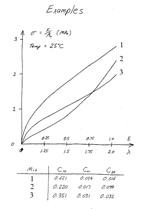
Popular Coefficients
It is popular to choose the following coefficients: \(C_{10}\), \(C_{01}\), and \(C_{20}\). These three lead to the following equation(s) to be curve-fit to experimental data.\[ \begin{eqnarray} \sigma_1 & = & \lambda_1 \Big\{ \big[ C_{10} + 2 \, C_{20} (I_1 - 3) \big] \big[ 2 \lambda_1 \big] + \big[ C_{01} \big] \big[ {-2 / \lambda_1^3 } \big] \Big\} + 2 \, D \, \epsilon_\text{Vol} \\ \\ \\ & = & 2 \, C_{10} \lambda_1^2 - 2 \, C_{01} {1 \over \lambda_1^2 } + 4 \, C_{20} \lambda_1^2 (\lambda_1^2 + \lambda_2^2 + \lambda_3^2 - 3) + 2 \, D \, \epsilon_\text{Vol} \end{eqnarray} \]
Likewise, the equations for \(\sigma_2\) and \(\sigma_3\) are
\[ \begin{eqnarray} \sigma_2 & = & 2 \, C_{10} \lambda_2^2 - 2 \, C_{01} {1 \over \lambda_2^2 } + 4 \, C_{20} \lambda_2^2 (\lambda_1^2 + \lambda_2^2 + \lambda_3^2 - 3) + 2 \, D \, \epsilon_\text{Vol} \\ \\ \\ \sigma_3 & = & 2 \, C_{10} \lambda_3^2 - 2 \, C_{01} {1 \over \lambda_3^2 } + 4 \, C_{20} \lambda_3^2 (\lambda_1^2 + \lambda_2^2 + \lambda_3^2 - 3) + 2 \, D \, \epsilon_\text{Vol} \\ \end{eqnarray} \]
Don't forget that the stresses here are Cauchy stresses, not engineering stresses.
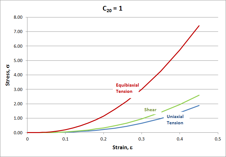
Keep in mind that there is no physical insight built into these equations! They are merely a collection of polynomials that happen to curve this way and that, in ways that are similar to the stress-strain curves one gets from actual laboratory tests on rubber test specimens. The equations also possess one additional key critical property. As will be seen shortly, they predict higher principal stresses for equibiaxial tension than plane strain tension, and then higher again against uniaxial tension.
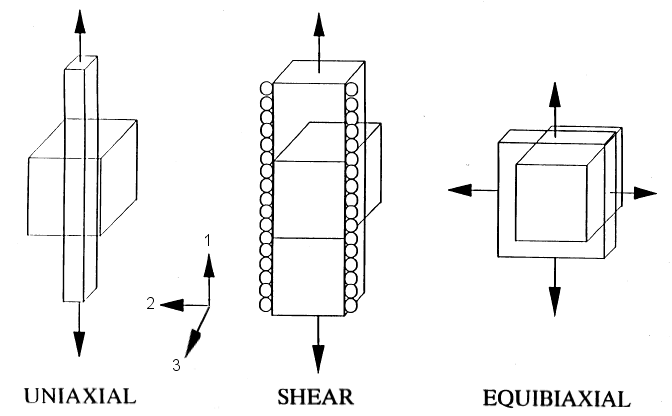
Specific Deformation Modes
Recall the three main deformation modes covered on the special strain topics page. These constitute the two extreme deformation modes, along with the plane strain tension mode midway between the two. Note that plane strain tension has the same principal values as the pure shear case when strains are small. For this reason, it is often compared to shear deformations.Developing Mooney-Rivlin equations for these special cases appears to be a very popular thing to do. There are a couple reasons for this. First, the deformation modes are (relatively) easily accomplished in lab tests, at least the uniaxial tension case is. The second reason is that the equations can be manipulated to eliminate the bulk modulus, which makes life a little easier. This will be demonstrated next.
The key to eliminating the bulk modulus for these three special cases is to recognize that \(\sigma_3 = 0\) in each. Therefore, one can subtract two equations from each other to accomplish \(\sigma_1 - \sigma_3\) as follows.
\[ \sigma_1 - \sigma_3 = 2 \, C_{10} (\lambda_1^2 - \lambda_3^2) + 2 \, C_{01} \left( {1 \over \lambda_3^2 } - {1 \over \lambda_1^2} \right) + 4 \, C_{20} (\lambda_1^2 - \lambda_3^2) (\lambda_1^2 + \lambda_2^2 + \lambda_3^2 - 3) \]
But \(\sigma_3 = 0\), so
\[ \sigma_1 = 2 \, C_{10} (\lambda_1^2 - \lambda_3^2) + 2 \, C_{01} \left( {1 \over \lambda_3^2 } - {1 \over \lambda_1^2} \right) + 4 \, C_{20} (\lambda_1^2 - \lambda_3^2) (\lambda_1^2 + \lambda_2^2 + \lambda_3^2 - 3) \]
An alternative popular form is obtained by dividing through by \(\lambda_1\) to obtain engineering stress. It is this form that is often used to determine the Mooney-Rivlin coefficients by fitting the equation(s) to experimental data.
\[ \sigma_1^\text{Eng} = 2 \, C_{10} \left( \lambda_1 - {\lambda_3^2 \over \lambda_1} \right) + 2 \, C_{01} \left( {1 \over \lambda_1 \lambda_3^2 } - {1 \over \lambda_1^3} \right) + 4 \, C_{20} \left( \lambda_1 - {\lambda_3^2 \over \lambda_1} \right) (\lambda_1^2 + \lambda_2^2 + \lambda_3^2 - 3) \]
Uniaxial Tension
Recall that for uniaxial tension in the \(1\) direction, incompressibility requires\[ \lambda_1 = \lambda \qquad \qquad \lambda_2 = \lambda_3 = {1 \over \sqrt{\lambda} } \]
Substituting these into the equation for engineering stress gives
\[ \sigma_\text{Uniaxial}^\text{Eng} = 2 C_{10} \left( \lambda - {1 \over \lambda^2 } \right) + 2 C_{01} \left( 1 - {1 \over \lambda^3} \right) + 4 \, C_{20} \left( \lambda - {1 \over \lambda^2 } \right) \left( \lambda^2 + {2 \over \lambda} - 3 \right) \]
Plane Strain Tension (Shear)
For this case\[ \lambda_1 = \lambda \qquad \qquad \lambda_2 = 1 \qquad \qquad \lambda_3 = {1 \over \lambda } \]
And the equation for stress is
\[ \sigma_{\begin{eqnarray}\text{Plane}\;\;\, \\ \text{Strain}\;\; \\ \text{Tension}\end{eqnarray}}^\text{Eng} = \; 2 \, C_{10} \left( \lambda - {1 \over \lambda^3 } \right) + 2 \, C_{01} \left( \lambda - {1 \over \lambda^3} \right) + 4 \, C_{20} \left( \lambda - {1 \over \lambda^3 } \right) \left( \lambda^2 + { 1 \over \lambda^2 } - 2 \right) \]
Equibiaxial Tension
For this case\[ \lambda_1 \; = \; \lambda_2 \; = \; \lambda \qquad \qquad \lambda_3 \; = \; {1 \over \lambda^2 } \]
And the stress is
\[ \sigma_\text{Equibiaxial}^\text{Eng} = 2 C_{10} \left( \lambda - {1 \over \lambda^5 } \right) + 2 C_{01} \left( \lambda^3 - {1 \over \lambda^3} \right) + 4 \, C_{20} \left( \lambda - {1 \over \lambda^5 } \right) \left( 2 \lambda^2 + {1 \over \lambda^4} - 3 \right) \]
Uniaxial Tension
This shows the basic curves for uniaxial tension when each coefficient is set to 1.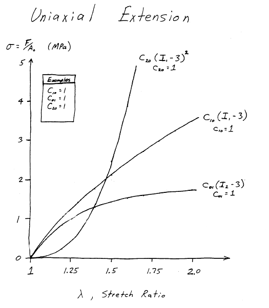
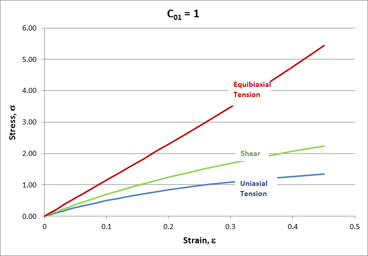
Stress-Strain Curves
For the case where \(C_{10} = 1\) and all other constants are zero...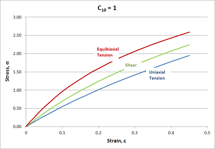
For the case where \(C_{01} = 1\) and all other constants are zero...
For the case where \(C_{20} = 1\) and all other constants are zero...
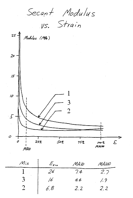
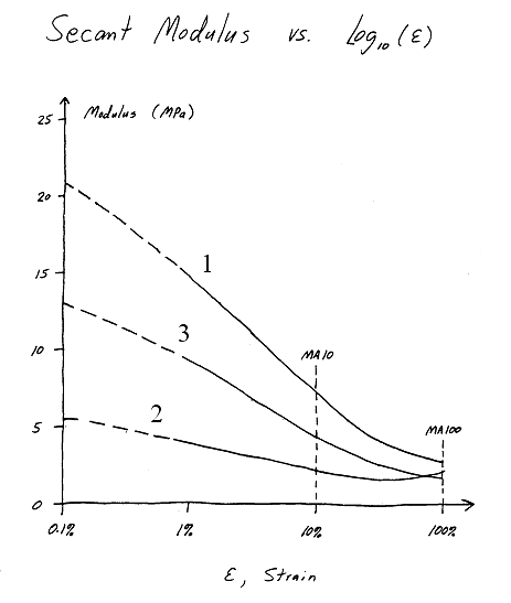
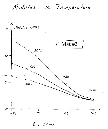
MA10 and MA100
MA10 and MA100 are secant moduli at 10% and 100% engineering strain under uniaxial tension conditions. \(\lambda = 1.10\) for MA10 and \(\lambda = 2.00\) for MA100. The way to compute MA10 from Mooney-Rivlin coefficients is to first calculate the stress at \(\lambda = 1.10\) and then divide that stress by \(\epsilon = 0.10\). The equation for uniaxial tension is\[ \sigma^\text{Eng} = 2 \, C_{10} \left( \lambda - {1 \over \lambda^2 } \right) + 2 \, C_{01} \left( 1 - {1 \over \lambda^3} \right) + 4 \, C_{20} \left( \lambda - {1 \over \lambda^2 } \right) \left( \lambda^2 + {2 \over \lambda} - 3 \right) \]
Insert \(\lambda = 1.10\) into the equation to get
\[ \sigma^\text{Eng}_\text{10%} = 0.547 \, C_{10} + 0.497 \, C_{01} + 0.031 C_{20} \]
And divide by 0.10 to get MA10.
\[ \text{MA10} \; = \; 5.47 \, C_{10} + 4.97 \, C_{01} + 0.31 \, C_{20} \]
And MA100 is
\[ \text{MA100} \; = \; 3.5 \, C_{10} + 1.75 \, C_{01} + 14 \, C_{20} \]
For reference, the slope at zero strain is the following
\[ E_{\epsilon=0} \; = \; \left. {d \sigma \over d \lambda}\right|_{\lambda=1} \; = \; 6 \, ( C_{10} + C_{01} ) \]
The \(C_{20}\) term has zero slope at \(\epsilon = 0\).
Experimental Data
Found on a Forum...
Problem with parameters in Mooney-Rivlin modelHello,
I want to use Mooney-Rivlin parametrs from the paper publish in the internet - they received parameters :
C10: 2.7507e-2
C01: 1.3077e-1
C11: 6.8027e-2
D: 4.8694e-2
My problem is :
Authors of these paper didn't mention what units of stress and strain they used to obtained the C10, C01, C11, D parameters. Is the units of input data of stress-strain important?