Introduction
This chapter on displacements and deformations is the heart of continuum mechanics. And this page and the next, which cover the deformation gradient, are the center of that heart. The deformation gradient is used to separate rigid body translations and rotations from deformations, which are the source of stresses.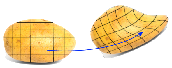
As is the convention in continuum mechanics, the vector \({\bf X}\) is used to define the undeformed reference configuration, and \({\bf x}\) defines the deformed current configuration. In each case, imagine that the (almost) square grid on the potato is displaced, rotated, and/or deformed.
Deformation Gradient
The deformation gradient \({\bf F}\) is the derivative of each component of the deformed \({\bf x}\) vector with respect to each component of the reference \({\bf X}\) vector. For \({\bf x} = {\bf x}({\bf X})\), then\[ F_{ij} \quad = \quad x_{i,j} \quad = \quad \frac{\partial x_i}{\partial X_j} \quad = \quad \left[ \matrix{ {\partial x_1 \over \partial X_1} & {\partial x_1 \over \partial X_2} & {\partial x_1 \over \partial X_3} \\ {\partial x_2 \over \partial X_1} & {\partial x_2 \over \partial X_2} & {\partial x_2 \over \partial X_3} \\ {\partial x_3 \over \partial X_1} & {\partial x_3 \over \partial X_2} & {\partial x_3 \over \partial X_3} } \right] \]
A slightly altered calculation is possible by noting that the displacement \({\bf u}\) of any point can be defined as
and this leads to \({\bf x} = {\bf X} + {\bf u}\), and
\[ {\bf F} \quad = \quad { \partial \over \partial {\bf X} } ({\bf X} + {\bf u}) \quad = \quad { \partial {\bf X} \over \partial {\bf X} } + { \partial {\bf u} \over \partial {\bf X} } \quad = \quad {\bf I} + { \partial {\bf u} \over \partial {\bf X} } \]
In tensor notation, this is written as
\[ F_{ij} = \delta_{ij} + u_{i,j} \]
Rigid Body Displacements

\[ \begin{eqnarray} x & = & X & + & 5 \\ y & = & Y & + & 2 \end{eqnarray} \]
In this case, \({\bf F} = {\bf I}\), is indicative of a lack of deformations. As will be shown next, it is also indicative of a lack of rotations. Clearly rigid body displacements do not appear in the deformation gradient. This is good because rigid body displacements don't contribute to stress, strain, etc.
Rigid Body Rotations
An example of a rigid body rotation is
These equations rotate an object counter-clockwise about the \(z\) axis. Notice how the minus sign is now in the \((1,2)\) slot instead of the \((2,1)\) slot as was the case for coordinate transformations. See this page on rotation matrices for an explanation.
In this case, \({\bf F}\) is
\[ {\bf F} = \left[ \matrix{ \cos \theta & -\sin \theta \\ \sin \theta & \;\;\;\; \cos \theta } \right] \]
Rotations alter the value of \({\bf F}\) so that it is no longer equal to \({\bf I}\) even though no deformations are present. This can lead to misinterpretations in which rigid body rotations are mistaken for deformations and strain. This is the main complicating factor in finite deformation mechanics. Unfortunately, it will get even worse when rotations and deformations are present at the same time.
Simple Deformations
Case 1 - Stretching

\[ \begin{eqnarray} x & = & 2.0 X \, & + & 0.0 \, Y \\ y & = & 0.0 X \, & + & 1.5 \, Y \end{eqnarray} \]
The deformation gradient is
\[ {\bf F} = \left[ \matrix{ 2.0 & 0.0 \\ 0.0 & 1.5 } \right] \]
Note that all off-diagonal components are zero. \(F_{11}\) reflects stretching in the x-direction and \(F_{22}\) reflects stretching in the y-direction.
Case 2 - Shear (with Rotation)
These equations shear the square as shown.
The deformation gradient is
\[ {\bf F} = \left[ \matrix{ 1.0 & 0.0 \\ 0.5 & 1.0 } \right] \]
The non-zero off-diagonal value reflects shear. The figure also shows that the square tends to rotate counter-clockwise. This is reflected in the deformation gradient by the fact that it is not symmetric.
Case 3 - Pure Shear
These equations shear the square with zero net rotation.
The deformation gradient is
\[ {\bf F} = \left[ \matrix{ 1.0 & 0.5 \\ 0.5 & 1.0 } \right] \]
The non-zero off-diagonal values mean that shearing is present. The fact that \({\bf F}\) is symmetric reflects that there is no net rotation. The zero net rotation arises from the fact that while the lower right area of the square tends to rotate counter-clockwise, the upper left area tends to rotate clockwise at the same time. Therefore, the net rotation for the square as a whole is zero.
General Deformations
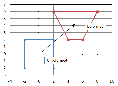
Consider the example where an object is transformed from a square to the position shown in the figure. The equations to do this are
\[ \begin{eqnarray} x & = & 1.300 X \, & - & 0.375 \, Y \\ y & = & 0.750 X \, & + & 0.650 \, Y \end{eqnarray} \]
and the corresponding deformation gradient is
\[ {\bf F} = \left[ \matrix{ 1.300 & -0.375 \\ 0.750 & \;\;\;0.650 } \right] \]
The object has clearly been stretched and rotated. But by how much? The rotation doesn't contribute to stress, but the deformation does. So it is necessary to partition the two mechanisms out of \({\bf F}\) in order to determine the stress and strain state.
The next page on polar decompositions will show how to do this. But for now, just accept that the following two-step process of deformation followed by rigid body rotation gets you there...
The first step is a 50% stretch in the x-direction and a 25% compression in the y-direction. This gets us from the \({\bf X}\) reference coordinates to the intermediate \({\bf x'}\) coordinates.
\[ \begin{eqnarray} x' & = & 1.50 X \, & + & 0.00 \, Y \\ y' & = & 0.00 X \, & + & 0.75 \, Y \end{eqnarray} \]
The second step is to rotate the \({\bf x'}\) intermediate configuration to the final \({\bf x}\) coordinates.
\[ \begin{eqnarray} x & \quad = \quad & x' \cos(30^\circ) \, & - & y' \sin(30^\circ) & \quad = \quad & 1.300 X \, & - & 0.375 \, Y \\ y & \quad = \quad & x' \sin(30^\circ) \, & + & y' \cos(30^\circ) & \quad = \quad & 0.750 X \, & + & 0.650 \, Y \end{eqnarray} \]
In matrix form,
\[ \left\{ \matrix{ x \\ y } \right\} = \left[ \matrix{ 0.866 & -0.500 \\ 0.500 & \;\;\;0.866 } \right] \left\{ \matrix{ x' \\ y' } \right\} \qquad \text{and} \qquad \left\{ \matrix{ x' \\ y' } \right\} = \left[ \matrix{ 1.50 & 0.00 \\ 0.00 & 0.75 } \right] \left\{ \matrix{ X \\ Y } \right\} \]
and the deformation gradient can be written as the product of two matrices: a rotation matrix, and a symmetric matrix describing the deformation.
\[ {\bf F} \quad = \quad \left[ \matrix{ 1.300 & -0.375 \\ 0.750 & \;\;\;0.650 } \right] \quad = \quad \left[ \matrix{ 0.866 & -0.500 \\ 0.500 & \;\;\;0.866 } \right] \left[ \matrix{ 1.50 & 0.00 \\ 0.00 & 0.75 } \right] \]
It is easy to see that the rotation matrix corresponds to a 30° rotation. The matrix product is commonly written as
\[ {\bf F} = {\bf R} \cdot {\bf U} \]
where \({\bf R}\) is the rotation matrix, and \({\bf U}\) is the right stretch tensor that is responsible for all the problems in life: stress, strain, fatigue, cracks, fracture, etc. Note that the process is read from right to left, not left to right. \({\bf U}\) is applied first, then \({\bf R}\).
This partitioning of the deformation gradient into the product of a rotation matrix and stretch tensor is known as a Polar Decomposition. The next page on Polar Decompositions will show how to do this for the general 3-D case.
Or Alternatively...
The deformed and rotated state could equally-well be arrived at by rotating it first, and then deforming it second. In this case, the reference configuration, \({\bf X}\), is first rotated by the same 30° angle to arrive at an intermediate configuration, \({\bf x'}\).
\[ \begin{eqnarray} x' & \quad = \quad & X \cos(30^\circ) & - & Y \sin(30^\circ) \\ y' & \quad = \quad & X \sin(30^\circ) & + & Y \cos(30^\circ) \end{eqnarray} \]
And then the intermediate configuration is deformed to arrive at the final, deformed state
\[ \begin{eqnarray} x & \quad = \quad & 1.313 x' \, & + & 0.325 \, y' \\ y & \quad = \quad & 0.325 x' \, & + & 0.938 \, y' \end{eqnarray} \]
The off-diagonal values reflect that the object is being sheared in addition to being stretched/compressed.
The deformation gradient can be written as
\[ {\bf F} \quad = \quad \left[ \matrix{ 1.300 & -0.375 \\ 0.750 & \;\;\;0.650 } \right] \quad = \quad \left[ \matrix{ 1.313 & 0.325 \\ 0.325 & 0.938 } \right] \left[ \matrix{ 0.866 & -0.500 \\ 0.500 & \;\;\;0.866 } \right] \]
This is commonly written as
\[ {\bf F} = {\bf V} \cdot {\bf R} \]
where \({\bf R}\) is the rotation matrix (same as before), and \({\bf V}\) is the left stretch tensor. This is also a polar decomposition.
Relationship Between V and U
It is relatively easy to develop a relationship between \({\bf V}\) and \({\bf U}\).Since \({\bf F} = {\bf V} \cdot {\bf R}\) and \({\bf F} = {\bf R} \cdot {\bf U}\), then
\[ {\bf V} \cdot {\bf R} = {\bf R} \cdot {\bf U} \]
and post-multiplying through by \({\bf R}^T\) gives
\[ {\bf V} \cdot {\bf R} \cdot {\bf R}^T = {\bf R} \cdot {\bf U} \cdot {\bf R}^T \]
\[ {\bf V} = {\bf R} \cdot {\bf U} \cdot {\bf R}^T \]
as the relationship between \({\bf V}\) and \({\bf U}\).
Alternatively, solving for \({\bf U}\) gives
\[ {\bf U} = {\bf R}^T \cdot {\bf V} \cdot {\bf R} \]
Verifying Relationship Between V and U
Recall that\[ \qquad {\bf V} = \left[ \matrix{ 1.313 & 0.325 \\ 0.325 & 0.938 } \right] \qquad {\bf R} = \left[ \matrix{ 0.866 & -0.500 \\ 0.500 & \;\;\;0.866 } \right] \qquad {\bf U} = \left[ \matrix{ 1.500 & 0.0 \\ 0.0 & 0.750 } \right] \]
Evaluating \( {\bf R} \cdot {\bf U} \cdot {\bf R}^T \) gives
\[ \begin{eqnarray} {\bf R} \cdot {\bf U} \cdot {\bf R}^T \quad & = & \quad \left[ \matrix{ 0.866 & -0.500 \\ 0.500 & \;\;\;0.866 } \right] \left[ \matrix{ 1.500 & 0.0 \\ 0.0 & 0.750 } \right] \left[ \matrix{ \;\;\; 0.866 & 0.500 \\ -0.500 & 0.866 } \right] \\ \\ \\ \quad & = & \quad \left[ \matrix{ 1.313 & 0.325 \\ 0.325 & 0.938 } \right] \end{eqnarray} \]
which confirms that \({\bf R} \cdot {\bf U} \cdot {\bf R}^T \) is indeed equal to \({\bf V}\).
Coordinate Mapping Example - Hourglassing
After much trial and error... the equations relating undeformed and deformed states are
\[ \begin{eqnarray} x & = & X + \frac{1}{4} X Y + 5 \\ \\ y & = & Y + 4 \end{eqnarray} \]
These equations can be checked by substituting the coordinates of any of the four corners of the undeformed square to arrive at the deformed coordinates.
Once the mapping equations are available, the deformation gradient is easy
\[ {\bf F} = \left[ \matrix{ 1 + \frac{1}{4} Y & \frac{1}{4} X \\ \\ 0 & 1 } \right] \]
The bottom row values of \(F_{21} = 0\) and \(F_{22} = 1\) mean that nothing is happening in the \(Y\) direction. All the action is in the \(X\) direction.
Of special note is the condition at the center of the square, at \((0,0)\). Inserting \((0,0)\) into the deformation gradient gives
\[ {\bf F} = \left[ \matrix{ 1 & 0 \\ 0 & 1 } \right] \] which is the identity matrix. This indicates that there is no deformation at all at the center of the square even though it is clearly deforming at every other location.
This effect is known as hourglassing in FE analyses and arises in 2-D quadrilateral and 3-D brick elements undergoing reduced integration. In such cases, element deformations are only evaluated at the center of the element. As a result, hourglass deformations are not detected and can grow uncontrollably.
V and U for Different Rigid Body Rotations
For an object that is stretched by 100% along the x-axis, but not rotated, the deformation gradient and polar decompositions are\[ \begin{eqnarray} {\bf F} & = & {\bf R} \cdot {\bf U} \\ \\ \left[ \matrix{ 2 & 0 \\ 0 & 1 } \right] & = & \left[ \matrix{ \cos 0^\circ & \!\!\!\!\text{-}\sin 0^\circ \\ \sin 0^\circ & \!\!\cos 0^\circ } \right] \left[ \matrix{ 2 & 0 \\ 0 & 1 } \right] \end{eqnarray} \]
And the \({\bf V} \cdot {\bf R}\) polar decomposition is
\[ \begin{eqnarray} {\bf F} & = & {\bf V} \cdot {\bf R} \\ \\ \left[ \matrix{ 2 & 0 \\ 0 & 1 } \right] & = & \left[ \matrix{ 2 & 0 \\ 0 & 1 } \right] \left[ \matrix{ \cos 0^\circ & \!\!\!\!\text{-}\sin 0^\circ \\ \sin 0^\circ & \!\!\cos 0^\circ } \right] \end{eqnarray} \]
Yes, when there is no rotation, \({\bf U}\), \({\bf V}\), and \({\bf F}\) are all the same. They must be.
If the object is stretched 100% along the direction that was originally parallel to the x-axis, and also rotated 90°, then the deformation gradient and polar decompositions are
\[ \begin{eqnarray} {\bf F} & = & {\bf R} \cdot {\bf U} \\ \\ \left[ \matrix{ 0 & \text{-}1 \\ 2 & \;0 } \right] & = & \left[ \matrix{ \cos 90^\circ & \!\!\!\!\text{-}\sin 90^\circ \\ \sin 90^\circ & \!\!\cos 90^\circ } \right] \left[ \matrix{ 2 & 0 \\ 0 & 1 } \right] \end{eqnarray} \]
And the \({\bf V} \cdot {\bf R}\) polar decomposition is
\[ \begin{eqnarray} {\bf F} & = & {\bf V} \cdot {\bf R} \\ \\ \left[ \matrix{ 0 & \text{-}1 \\ 2 & \;0 } \right] & = & \left[ \matrix{ 1 & 0 \\ 0 & 2 } \right] \left[ \matrix{ \cos 90^\circ & \!\!\!\!\text{-}\sin 90^\circ \\ \sin 90^\circ & \!\!\cos 90^\circ } \right] \end{eqnarray} \]
The \({\bf U}\) stretch tensor hasn't changed between the 0° and 90° rotation example, however the \({\bf V}\) stretch tensor has (as well as \({\bf F}\)). \({\bf V}\)'s components always correspond to deformations that are described after the rotation takes place.
Discussion
Everyone always wants to know, "But which one, \({\bf R}\cdot{\bf U}\) or \({\bf V}\cdot{\bf R}\) should I use?" Again, neither is more or less correct than the other. Both describe the exact same deformed state. The usual determining factor is whether one prefers to think of the deformations as occurring in the reference orientation, or in the final rotated state. Nevertheless, the usual preference is to use \({\bf F} = {\bf R}\cdot{\bf U}\) because it is normally easier to relate the strains back to the undeformed orientation. This leads to the Green strain definition that is popular in tire mechanics and will be discussed in a few more pages.
One last example: One could assume that an object is stretched in the x-direction, and then rotated 90°. In this case, the \(\epsilon_{xx}\) strain is non-zero. Alternatively, one could just as well assume that the object was rotated 90° first, then stretched in the vertical direction, giving a non-zero \(\epsilon_{yy}\) strain. If all you've got is the final deformed shape to work with, then either path works.
And one last note: All this hints at a larger issue. It is the question, "Of all the definitions of strain, which is the best?" The answer is, "Neither is necessarily more or less correct than any other." Some are just more convenient than others for a given application. We will come back to this topic later.