Introduction
The polar decomposition concept was introduced on the previous deformation gradient page. In it, we saw through example that \({\bf F}\) can be written as either \({\bf R} \cdot {\bf U}\) or \({\bf V} \cdot {\bf R}\). In each case, \({\bf R}\) is the rotation matrix, and \({\bf U}\) and \({\bf V}\) are symmetric matrices describing the deformations.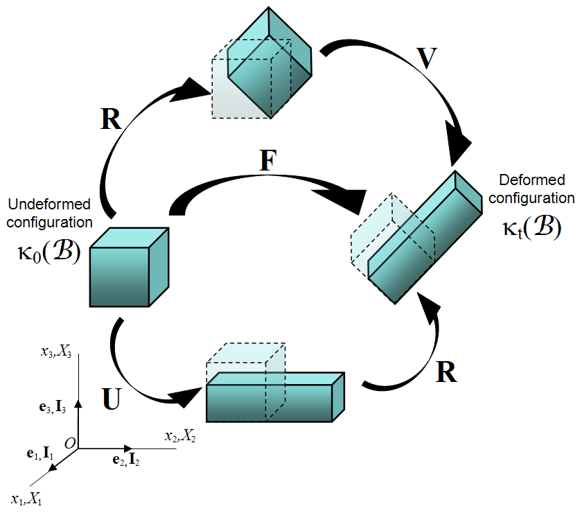
The purpose of this page is to show how to compute a polar decomposition in the general 3-D case. That process will introduce another new concept: the square root of a matrix. But first...
Product with Transpose
Recall from this page on matrices that the product of a matrix with its transpose is always a symmetric matrix. Plugging the polar decomposition into this gives a rather surprising result.\[ {\bf F}^T \! \cdot {\bf F} \quad = \quad \left( {\bf R} \cdot {\bf U} \right)^T \cdot \left( {\bf R} \cdot {\bf U} \right) \quad = \quad {\bf U}^T \cdot {\bf R}^T \cdot {\bf R} \cdot {\bf U} \]
But as with \({\bf Q}\), here \({\bf R}^T\) is the inverse of \({\bf R}\) (This is discussed on the next page). So
\[ {\bf R}^T \cdot {\bf R} \quad = \quad {\bf R}^{-1} \cdot {\bf R} \quad = \quad {\bf I} \]
And \({\bf F}^T \! \cdot {\bf F}\) reduces to
\[ {\bf F}^T \! \cdot {\bf F} \quad = \quad \left( {\bf R} \cdot {\bf U} \right)^T \cdot \left( {\bf R} \cdot {\bf U} \right) \quad = \quad {\bf U}^T \! \cdot {\bf R}^T \cdot {\bf R} \cdot {\bf U} \quad = \quad {\bf U}^T \! \cdot {\bf U} \]
The result is called the "Right Cauchy-Green Deformation Tensor," and sometimes represented by \({\bf C}\), but I don't like this because it hides the true physics behind the letter \({\bf C}\), which is \({\bf U}^T \! \cdot {\bf U}\). So I won't be using it.
\[ {\bf F} \cdot {\bf F}^T \quad = \quad \left( {\bf V} \cdot {\bf R} \right) \cdot \left( {\bf V} \cdot {\bf R} \right)^T \quad = \quad {\bf V} \cdot {\bf R} \cdot {\bf R}^T \! \cdot {\bf V}^T \quad = \quad {\bf V} \cdot {\bf V}^T \]
And this result is called the "Left Cauchy-Green Deformation Tensor," and sometimes represented by \({\bf B}\), but I don't like this because it also hides the true physics behind the letter \({\bf B}\), which is \({\bf V} \cdot {\bf V}^T\). So I won't be using it either.
The surprising result here is that the rotation matrix, \({\bf R}\), has been eliminated from the problem in each case. But a new challenge has been introduced, that of finding \({\bf U}\) from \(({\bf U}^T \! \cdot {\bf U})\) and \({\bf V}\) from \(({\bf V} \cdot {\bf V}^T)\). This is the source of the need to compute square roots of matrices. Recall that \({\bf U}\) and \({\bf V}\) are both symmetric, so \( {\bf U} = {\bf U}^T \) and \( {\bf U}^T \cdot {\bf U} = {\bf U} \cdot {\bf U} \). Likewise \( {\bf V} = {\bf V}^T \) and \( {\bf V} \cdot {\bf V}^T = {\bf V} \cdot {\bf V} \). Finally, \( {\bf U} \cdot {\bf U} \) is sometimes written as \( {\bf U}^2 \) and \( {\bf V} \cdot {\bf V} \) is sometimes written as \( {\bf V}^2 \).
Determination of R & U

\[ \begin{eqnarray} x & = & 1.300 X \, & - & 0.375 \, Y \\ \\ y & = & 0.750 X \, & + & 0.650 \, Y \end{eqnarray} \]
and the deformation gradient is
\[ {\bf F} = \left[ \matrix{ 1.300 & -0.375 \\ 0.750 & \;\;\;0.650 } \right] \]
So \( {\bf F}^T \! \cdot {\bf F}\) is
\[ {\bf F}^T \! \cdot {\bf F} \quad = \quad \left[ \matrix{ \;\;\; 1.300 & 0.750 \\ -0.375 & 0.650 } \right] \left[ \matrix{ 1.300 & -0.375 \\ 0.750 & \;\;\;0.650 } \right] \quad = \quad \left[ \matrix{ 2.250 & 0.000 \\ 0.000 & 0.563 } \right] \quad = \quad {\bf U}^T \! \cdot {\bf U} \]
This is the simplest of all scenarios - a diagonal matrix. In this case, the \({\bf U}\) matrix is just the square-roots of the diagonal values.
\[ {\bf U} \quad = \quad \left[ \matrix{ \sqrt{2.25} & 0.0 \\ 0.0 & \sqrt{0.563} } \right] \quad = \quad \left[ \matrix{ 1.5 & 0.0 \\ 0.0 & 0.75 } \right] \]
which is exactly the \({\bf U}\) matrix result from the previous page. Once \({\bf U}\) is determined, the final step is to multiply \({\bf F}\) through by the inverse of \({\bf U}\) to get \({\bf R}\).
\[ {\bf F} \cdot {\bf U}^{-1} \quad = \quad {\bf R} \cdot {\bf U} \cdot {\bf U}^{-1} \quad = \quad {\bf R} \]
And the inverse of \({\bf U}\) is very simple in this case because it is diagonal.
\[ {\bf U}^{-1} \quad = \quad \left[ \matrix{ 0.667 & 0.0 \\ 0.0 & 1.333 } \right] \]
So \({\bf R}\) is
\[ {\bf R} \quad = \quad {\bf F} \cdot {\bf U}^{-1} \quad = \quad \left[ \matrix{ 1.300 & -0.375 \\ 0.750 & \;\;\;0.650 } \right] \left[ \matrix{ 0.667 & 0.0 \\ 0.0 & 1.333 } \right] \quad = \quad \left[ \matrix{ 0.866 & -0.500 \\ 0.500 & \;\;\;0.866 } \right] \]
This concludes this example of determining \({\bf R}\) and \({\bf U}\) from a deformation matrix, \({\bf F}\). However, it was deceptively simple in this case because \({\bf U}\) was a diagonal matrix, i.e., no shear. The next example will show the more typical, and much more complex case of performing a polar decomposition when shear is present in the problem.
Determination of V & R

\[ \begin{eqnarray} x & = & 1.300 X \, & - & 0.375 \, Y \\ \\ y & = & 0.750 X \, & + & 0.650 \, Y \end{eqnarray} \]
This time, performing the \({\bf V} \cdot {\bf R}\) decomposition begins with \( {\bf F} \cdot {\bf F}^T\).
\[ {\bf F} \cdot {\bf F}^T \quad = \quad \left[ \matrix{ 1.300 & -0.375 \\ 0.750 & \;\;\;0.650 } \right] \left[ \matrix{ \;\;\; 1.300 & 0.750 \\ -0.375 & 0.650 } \right] \quad = \quad \left[ \matrix{ 1.831 & 0.731 \\ 0.731 & 0.985 } \right] \quad = \quad {\bf V}\cdot {\bf V}^T \]
This is the more common situation in which the resulting matrix is not diagonal. This greatly complicates the process of finding its square root. As was the case with \({\bf U}\), recall that \({\bf V}\) is also symmetric, so \( {\bf V} = {\bf V}^T \) and \( {\bf V} \cdot {\bf V}^T = {\bf V} \cdot {\bf V} \).
Finding Square Roots of (Symmetric) Matrices
The steps are as follows:
- Transform the symmetric matrix to its principal orientation
- Take the square roots of the diagonal components
- Rotate back to the original orientation
\[ \tan 2 \theta = \left( {2 a_{12} \over a_{11} - a_{22} } \right) = \left( {2 * 0.731 \over 1.831 - 0.985 } \right) \quad \longrightarrow \quad \theta = 30^\circ \]
Applying the 30° rotation to \({\bf V} \cdot {\bf V}^T\) is done as follows
\[ \left[ \matrix{\;\;\; \cos 30^\circ & \sin 30^\circ \\ -\sin 30^\circ & \cos 30^\circ } \right] \left[ \matrix{1.831 & 0.731 \\ 0.731 & 0.985 } \right] \left[ \matrix{\cos 30^\circ & -\sin 30^\circ \\ \sin 30^\circ & \;\;\; \cos 30^\circ } \right] = \left[ \matrix{2.250 & 0.0 \\ 0.0 & 0.563 } \right] \]
which also should not be a surprise that the principal values of \({\bf V} \cdot {\bf V}^T\) are the same as those of \({\bf U}^T \cdot {\bf U}\). So the transformed \({\bf V'}\) matrix is
\[ {\bf V'} \quad = \quad \left[ \matrix{ \sqrt{2.25} & 0.0 \\ 0.0 & \sqrt{0.563} } \right] \quad = \quad \left[ \matrix{ 1.5 & 0.0 \\ 0.0 & 0.75 } \right] \]
The final step is to transform this result back by -30° to the original orientation.
\[ {\bf V} \quad = \quad \left[ \matrix{\;\;\; \cos (\text{-}30^\circ) & \sin (\text{-}30^\circ) \\ -\sin (\text{-}30^\circ) & \cos (\text{-}30^\circ) } \right] \left[ \matrix{1.5 & 0.0 \\ 0.0 & 0.75 } \right] \left[ \matrix{\cos (\text{-}30^\circ) & -\sin (\text{-}30^\circ) \\ \sin (\text{-}30^\circ) & \;\;\; \cos (\text{-}30^\circ) } \right] = \left[ \matrix{1.313 & 0.325 \\ 0.325 & 0.938 } \right] \]
And we arrive back at the original \({\bf V}\) matrix applied on the previous page. (Amazing how that works out!)
As a check of the square-root process...
\[ {\bf V} \cdot {\bf V} \quad = \quad \left[ \matrix{1.313 & 0.325 \\ 0.325 & 0.938 } \right] \left[ \matrix{1.313 & 0.325 \\ 0.325 & 0.938 } \right] = \left[ \matrix{1.831 & 0.731 \\ 0.731 & 0.985 } \right] \]
So this is correct.
Note that one thing that is not correct is to square each individual term of a matrix.
\[ \left[ \matrix{1.313^2 & 0.325^2 \\ 0.325^2 & 0.938^2 } \right] = \left[ \matrix{1.724 & 0.106 \\ 0.106 & 0.880 } \right] \ne \left[ \matrix{1.831 & 0.731 \\ 0.731 & 0.985 } \right] \]
\[ {\bf V}^{-1} \cdot {\bf F} \quad = \quad {\bf V}^{-1} \cdot {\bf V} \cdot {\bf R} \quad = \quad {\bf R} \]
The inverse of \({\bf V}\) can be computed using this page.
\[ {\bf V}^{-1} \quad = \quad \left[ \matrix{ \;\;\; 0.833 & -0.289 \\ -0.289 & \;\;\; 1.166 } \right] \]
And \({\bf R}\) is
\[ {\bf R} \quad = \quad {\bf V}^{-1} \cdot {\bf F} \quad = \quad \left[ \matrix{ \;\;\; 0.833 & -0.289 \\ -0.289 & \;\;\; 1.166 } \right] \left[ \matrix{ 1.300 & -0.375 \\ 0.750 & \;\;\;0.650 } \right] \quad = \quad \left[ \matrix{ 0.866 & -0.500 \\ 0.500 & \;\;\;0.866 } \right] \]
Which is the correct result... again.
This concludes the example of determining \({\bf V}\) and \({\bf R}\) from a deformation matrix, \({\bf F}\).
Review
\[ \begin{eqnarray} x & = & 1.300 X \, & - & 0.375 \, Y \\ \\ y & = & 0.750 X \, & + & 0.650 \, Y \end{eqnarray} \]
The deformation gradient is
\[ {\bf F} = \left[ \matrix{ 1.300 & -0.375 \\ 0.750 & \;\;\;0.650 } \right] \]
And this can be partitioned into
\[ {\bf F} \quad = \quad {\bf R} \cdot {\bf U} \quad = \quad \left[ \matrix{ 0.866 & -0.500 \\ 0.500 & \;\;\;0.866 } \right] \left[ \matrix{ 1.50 & 0.0 \\ 0.0 & 0.75 } \right] \]
Or alternatively
\[ {\bf F} \quad = \quad {\bf V} \cdot {\bf R} \quad = \quad \left[ \matrix{ 1.313 & 0.325 \\ 0.325 & 0.938 } \right] \left[ \matrix{ 0.866 & -0.500 \\ 0.500 & \;\;\;0.866 } \right] \]
In each case, the rotation is the same (because it must be). It's important to understand that the deformations are the same also. They just appear to be different because one is imposed before the object is rotated, the other after. To me, the advantage of the \({\bf R} \cdot {\bf U}\) decomposition, is that one can easily identify the deformations because they are applied to the underformed, unrotated, un-anythinged object. So one does not need to know how much the object rotated before knowing which directions on it were deformed.
3-D Example
\[ \begin{eqnarray} x & = & X + 2 Y \sin t + 0.5 Z \\ \\ y & = & -0.333 X + Y - Z \sin t \\ \\ z & = & X^2 \sin 2t + 1.5 Z \end{eqnarray} \]
so the deformation gradient is
\[ {\bf F} = {\partial \, x_i \over \partial X_j} = \left[ \matrix{ 1 & 2 \sin t & 0.5 \\ -0.333 & 1 & -\sin t \\ 2 X \sin 2t & 0 & 1.5 } \right] \]
And the question is, "What are the conditions at \({\bf X} = (1, 1, 1)\) at \(t = \text{0.25 sec}\)?"
Substituting the time and position coordinates in gives
\[ {\bf F} = {\partial \, x_i \over \partial X_j} = \left[ \matrix{ 1 & 0.495 & 0.5 \\ -0.333 & 1 & \; -0.247 \\ \;\;\; 0.959 & 0 & 1.5 } \right] \]
Begin the process by premultiplying \({\bf F}\) by its transpose. This page on matrix multiplication can be used to multiply the matrices.
\[ {\bf F}^T \cdot {\bf F} = \left[ \matrix{ 2.031 & 0.162 & 2.021 \\ 0.162 & 1.245 & 0 \\ 2.021 & 0 & 2.561 } \right] = {\bf U}^T \cdot {\bf U} \]
The next step is to find an orientation (i.e., a transformed coordinate system) that makes the result a diagonal matrix so that the square roots can be taken. This page on eigenvalues and eigenvectors can do that.
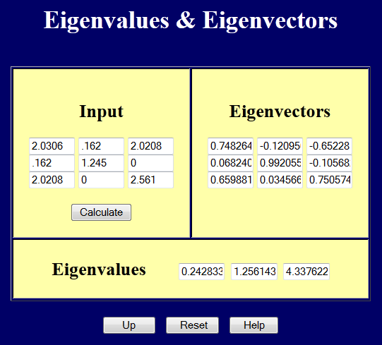
It reports that the principal values (eigenvalues) of \({\bf U}^T \! \cdot {\bf U}\) are
\[ {\bf U}'^2 = \left[ \matrix{ 0.243 & 0 & 0 \\ 0 & 1.256 & 0 \\ 0 & 0 & 4.338 } \right] \]
and the transformation matrix, \({\bf Q}\), used to obtain this is
\[ {\bf Q} = \left[ \matrix{ 0.748 & -0.121 & -0.652 \\ 0.068 & \;\;\;0.992 & -0.106 \\ 0.660 & \;\;\;0.035 & \;\;\;0.751 } \right] \]
The next step is to take the square root of the diagonal elements of \({\bf U}'^2\) to get
\[ {\bf U}' = \left[ \matrix{ 0.493 & 0 & 0 \\ 0 & 1.121 & 0 \\ 0 & 0 & 2.083 } \right] \]
and transform it back to the original coordinate system. There is in fact a relatively easy way to do this. It is
\[ {\bf U} = {\bf Q}^T \cdot {\bf U}' \cdot {\bf Q} \]
Multiplying this out gives
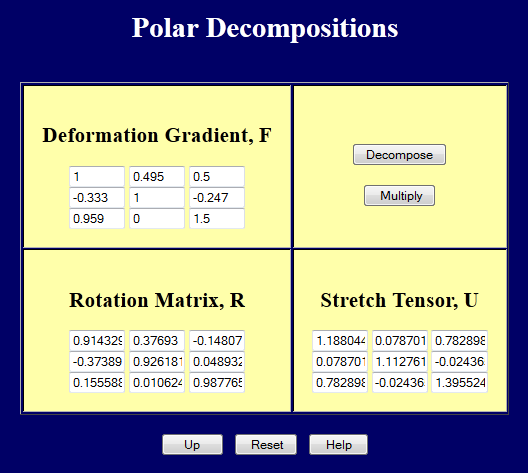
\[ {\bf U} = \left[ \matrix{ 1.188 & \;\;\;0.079 & \;\;\;0.783 \\ 0.079 & \;\;\;1.113 & -0.024 \\ 0.783 & -0.024 & \;\;\;1.396 } \right] \]
This shows that there is a lot of stretching in the \(Z\) direction, a little less in the \(X\) and \(Y\) directions, and a lot of shear in the \(X-Z\) direction.
The inverse of \({\bf U}\) is needed next. This page can calculate inverses. The result is
\[ {\bf U}^{-1} = \left[ \matrix{ \;\;\;1.349 & -0.112 & -0.759 \\ -0.112 & \;\;\;0.908 & \;\;\;0.079 \\ -0.759 & \;\;\;0.079 & \;\;\;1.144 } \right] \]
and finally, \({\bf R} = {\bf F} \cdot {\bf U}^{-1}\)
\[ {\bf R} = {\bf F} \cdot {\bf U}^{-1} = \left[ \matrix{ \;\;\;0.914 & 0.377 & -0.148 \\ -0.374 & 0.926 & \;\;\;0.049 \\ \;\;\;0.156 & 0.011 & \;\;\;0.988 } \right] \]
Or one could simply use this web page to compute the \({\bf R} \cdot {\bf U}\) decomposition.
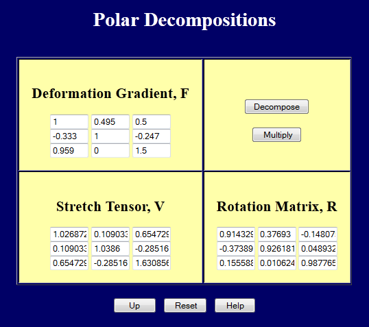
Or use this web page to compute the \({\bf V} \cdot {\bf R}\) decomposition.
Iterative Algorithm for Polar Decompositions
I recently learned of a most remarkable shortcut for performing polar decompositions that bypasses all the complexity of computing square roots of matrices. The method is iterative, and though it does require inverses and transposes, it is still considerably simpler than taking square roots. It relies on the following iterative formula to begin with the deformation gradient, \({\bf F}\), and arrive at the rotation matrix, \({\bf R}\).\[ {\bf A}_{n+1} = {1 \over 2} \left( {\bf A}_n + {\bf A}_n^{-T} \right) \]
\({\bf F}\) is inserted into the formula at the \({\bf A}_n\) locations, and \({\bf A}_{n+1}\) is computed. Then \({\bf A}_{n+1}\) is re-inserted back into the formula as \({\bf A}_n\) and a new \({\bf A}_{n+1}\) is calculated. After a few iterations, the output \({\bf A}_{n+1}\) matrix will be the same as the input \({\bf A}_n\) matrix. At this point, you will have the rotation matrix, \({\bf R}\). You can then pre or post multiply \({\bf F}\) by \({\bf R}^{-1}\) to obtain \({\bf U}\) or \({\bf V}\).
Let's return to the deformation gradient in the 3-D example above and apply the iterative formula to it to see the algorithm in action. Recall that \({\bf F}\) was
\[ {\bf F} = \left[ \matrix{ 1 & 0.495 & 0.5 \\ -0.333 & 1 & \; -0.247 \\ \;\;0.959 & 0 & 1.5 } \right] \]
The transpose of the inverse of \({\bf F}\) is \[ {\bf F}^{-T} = \left[ \matrix{ \;\;1.304 & 0.228 & -0.834 \\ -0.645 & 0.887 & \;\;0.413 \\ -0.541 & 0.070 & \;\;1.012 } \right] \]
and inserting into the formula gives
\[ \begin{eqnarray} {\bf A}_1 & = & {1 \over 2} \left( {\bf F} + {\bf F}^{-T} \right) \\ \\ & = & {1 \over 2} \left( \, \left[ \matrix{ 1 & 0.495 & 0.5 \\ -0.333 & 1 & \; -0.247 \\ \;\;0.959 & 0 & 1.5 } \right] + \left[ \matrix{ \;\;1.304 & 0.228 & -0.834 \\ -0.645 & 0.887 & \;\;0.413 \\ -0.541 & 0.070 & \;\;1.012 } \right] \, \right) \\ \\ & = & \left[ \matrix{ \;\;1.152 & 0.362 & -0.167 \\ -0.489 & 0.944 & \;\;0.083 \\ -0.209 & 0.035 & \;\;1.256 } \right] \end{eqnarray} \]
Repeating the process gives
\[ \begin{eqnarray} {\bf A}_2 & = & {1 \over 2} \left( {\bf A}_1 + {\bf A}_1^{-T} \right) \\ \\ & = & \left[ \matrix{ \;\;\;0.939 & 0.375 & -0.149 \\ -0.386 & 0.927 & \;\;0.052 \\ \;\;\;0.162 & 0.013 & \;\;1.017 } \right] \end{eqnarray} \]
and the next iteration...
\[ \begin{eqnarray} {\bf A}_3 & = & {1 \over 2} \left( {\bf A}_2 + {\bf A}_2^{-T} \right) \\ \\ & = & \left[ \matrix{ \;\;\;0.915 & 0.377 & -0.148 \\ -0.374 & 0.926 & \;\;0.049 \\ \;\;\;0.156 & 0.011 & \;\;0.988 } \right] \end{eqnarray} \]
\[ \begin{eqnarray} {\bf A}_4 & = & {1 \over 2} \left( {\bf A}_3 + {\bf A}_3^{-T} \right) \\ \\ & = & \left[ \matrix{ \;\;\;0.914 & 0.377 & -0.148 \\ -0.374 & 0.926 & \;\;0.049 \\ \;\;\;0.156 & 0.011 & \;\;0.988 } \right] \end{eqnarray} \]
It is clear that the process has converged, so the resulting matrix is \({\bf R}\). And it does match the rotation matrix computed above in the 3-D example. Its inverse can now be pre or post multiplied by \({\bf F}\) to obtain \({\bf U}\) or \({\bf V}\).