Introduction
Alas, such is not the case with Fourier transforms. In 30 years of working in acoustics, dynamic material testing, and vibrations, I have never, ever seen any topic provoke more apocalyptic levels of debate and outrage among technical types than the Fourier transform.
This tool must get misused and misinterpreted by more people than anything I've ever seen. These poor souls are ready to fight to the death over their erroneous conclusions. They don't want to hear that they are adding
So herewith, my attempt to save their immortal souls....
After a brief detour into the areas of background and motivation, we begin the first stage of exorcism with.... regressions.
Background
Fourier transforms and spectral analysis are motivated by the fact that deformations in a tire are periodic, repeating with each and every rotation. But while the deformations are periodic, they are not simple sinusoids. They are pulses in which all the action takes place during the short period of contact with the road. This is evident in the figure below, which shows the principal strains, as well as max and secondary shear strains for a tread block rolling through contact. It is clear that these traces are not straight-forward sinusoids. Therefore, Fourier analysis of the data is not trivial. And therein lies the challenge.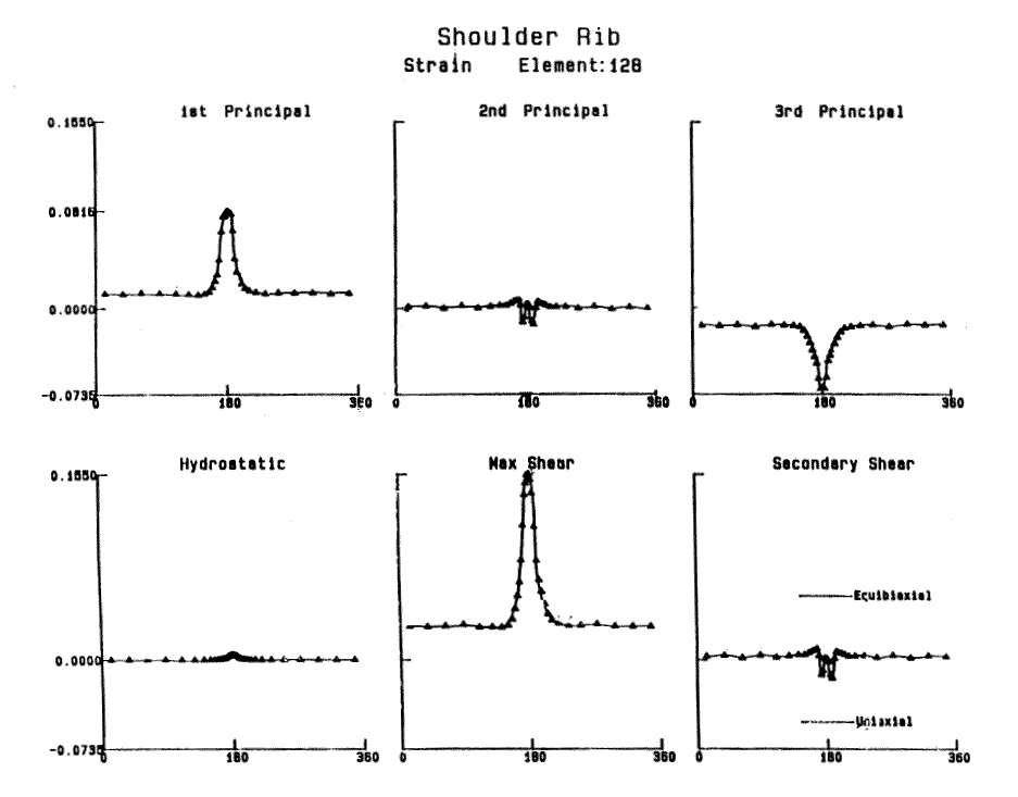
Regression
For example, just because an FFT of vibration data produces a harmonic at some given frequency, does NOT necessarily mean that the object was actually vibrating at that frequency. You cannot blindly accept such results without additional scrutiny. This is especially true of periodic data such as from tires, rotating machinery, helicopters, etc. These scenarios are the focus of this page. All have a clearly identifiable periodic aspect (or two) that is driving the problem.
Sadly, FFTs are seldom, if ever, presented as being regression curve-fits. They are usually presented as yet another obtuse mathematical process that converts time data into frequency data. But their subtle properties are not communicated.
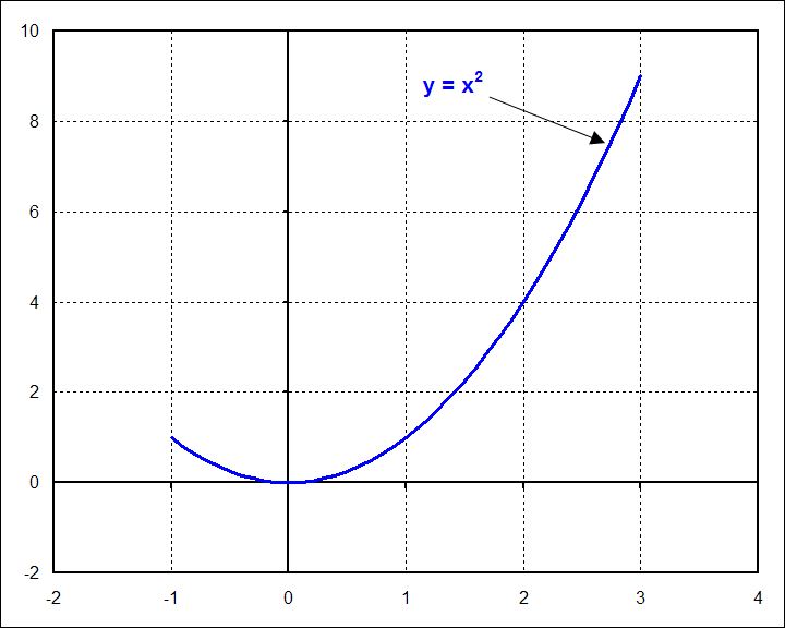
So let's start with an example of linear regression of a quadratic function in order to demonstrate the important fundamental principles. The function in the graph below is \(y = x^2\), plotted from \(x = -1\) to \(x = 3\).
Now fit a line, \(y = Ax + B\), to the function. This is done by choosing \(A\) and \(B\) such that the following integral is minimized. It represents the error, hence the \(E\), in fitting the line to the function. At each point, the two functions are subtracted from each other to obtain the difference, which is then squared so the result is always positive, and then added-up through the integration process.
\[ E = \int_{-1}^3 \left[ \left( x^2 \right) - \left( A x + B \right) \right]^2 dx \]
This is minimized by taking the derivatives with respect to \(A\) and \(B\) and setting them equal to zero. This gives two simultaneous equations that are solved for \(A\) and \(B\).
\[ \begin{eqnarray} {\partial E \over \partial A} & = & 2 \int_{-1}^3 A x^2 + B x - x^3 dx & = & 0 \\ \\ \\ {\partial E \over \partial B} & = & 2 \int_{-1}^3 A x + B - x^2 dx & = & 0 \end{eqnarray} \]
Writing this out a little more explicitly (and dropping the 2 from both equations) gives
\[ \begin{eqnarray} A \int_{-1}^3 x^2 dx + B \int_{-1}^3 x \, dx - \int_{-1}^3 x^3 dx & = & 0 \\ \\ \\ A \int_{-1}^3 x \, dx + B \int_{-1}^3 dx - \int_{-1}^3 x^2 dx & = & 0 \end{eqnarray} \]
Evaluating the integrals gives
\[ \begin{eqnarray} 9{1\over3} A + 4 \, B & = & 20 \\ \\ 4 \, A + 4 \, B & = & 9{1\over3} \end{eqnarray} \]
Solving for \(A\) and \(B\) gives \(A = 2\) and \(B = {1\over3}\). The graph of this is shown below.
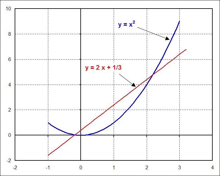
So far, so good. But now comes the misinterpretations. They arise from the linear regression we just obtained, which produced a line with slope equal to 2.0. These include (i) \(y = x^2\) has a straight component because otherwise the linear function would not have fit it, (ii) it has a linear component because otherwise the \(2x\) term would not have appeared, and (iii) \(y = x^2\) has a slope equal 2.0 because \(A = 2.0\). Of course, all of these conclusions are ridiculously wrong. And the example is simple enough that this is evident.
Alternatively, we could have done the opposite. We could have fit the quadratic function to the line and declared that the line must therefore have a curvy quadratic aspect to it because the quadratic function fit it. Hopefully, this is equally absurd. Yet, these are exactly the types of incorrect conclusions that are reached concerning Fourier transforms.
Recall that it was claimed up above that an FFT is nothing more than a curve-fit. It is in fact just a multivariable, linear regression.
Fourier Transforms
A Fourier transform is nothing more than the curve-fit of a collection of sine and cosine functions to some data. Those sine and cosine functions are\[ y = A_o + A_1 \cos ({ 2 \pi x \over L}) + B_1 \sin ({ 2 \pi x \over L}) + A_2 \cos ({ 4 \pi x \over L}) + B_2 \sin ({ 4 \pi x \over L}) + A_3 \cos ({ 6 \pi x \over L}) + B_3 \sin ({ 6 \pi x \over L}) + ... \]
The entire summation can be written compactly as
\[ y = \sum_{n=0}^N A_n \cos ({ 2 \pi n x \over L}) + \sum_{n=0}^N B_n \sin ({ 2 \pi n x \over L}) \]
or alternatively as
\[ y = \sum_{n=0}^N A'\!_n \cos ({ 2 \pi n x \over L} - \phi_n) \]
which more explicitly shows that each trig function is scaled vertically by \(A'\!_n\) and translated left/right by \(\phi_n\) until it best fits the data. The \(A'\!_n\) here equals \(\sqrt{A_n^2 + B_n^2}\), and \(\tan(\phi_n) = (B_n/A_n)\).
Plots of Fourier Transforms
\[ y = \sum_{n=0}^N A'\!_n \cos ({ 2 \pi n x \over L} - \phi_n) \]
Applying the same minimization process as the above quadratic example leads to
\[ E = \int_{x_1}^{x_2} \left[ f(x) - \left( \sum_{n=0}^N A_n \cos ({ 2 \pi n x \over L}) + \sum_{n=0}^N B_n \sin ({ 2 \pi n x \over L}) \right) \right]^2 dx \]
Taking the derivative with respect to \(A_n\) for a specific \(n\), call it \(n^*\), or \(A_{n^*}\) and setting it equal to zero gives
\[ {\partial E \over \partial A_{n^*}} = \int_{x_1}^{x_2} 2 \left[ f(x) - \sum_{n=0}^N A_n \cos ({ 2 \pi n x \over L}) - \sum_{n=0}^N B_n \sin ({ 2 \pi n x \over L}) \right] \cos ({ 2 \pi {n^*} x \over L}) \, dx = 0 \]
Some rearrangement gives
\[ \int_{x_1}^{x_2} f(x) \cos ({ 2 \pi {n^*} x \over L}) \, dx = \sum_{n=0}^N \int_{x_1}^{x_2} A_n \cos ({ 2 \pi n x \over L}) \cos ({ 2 \pi {n^*} x \over L}) \, dx + \sum_{n=0}^N \int_{x_1}^{x_2} B_n \sin ({ 2 \pi n x \over L}) \cos ({ 2 \pi {n^*} x \over L}) \, dx \]
Note that the integrals on the RHS do not contain the function, \(f(x)\). They are all completely determinate. The amazing thing is that all but one of them are zero. The only one that is not is
\[ \int_{x_1}^{x_2} A_n \cos ({ 2 \pi n x \over L}) \cos ({ 2 \pi {n^*} x \over L}) \, dx \]
for the case where \(n = n^*\). It equals \(A_n L / 2\) where \(L = x_2 - x_1\). So this gives
\[ \int_{x_1}^{x_2} f(x) \cos ({ 2 \pi {n^*} x \over L}) \, dx = {A_n L \over 2} \]
The \(*\) can now be dropped from \(n^*\) (because \(n = n^*\) ). And solving for \(A_n\) gives
\[ A_n = {2 \over L} \int_{x_1}^{x_2} f(x) \cos ({ 2 \pi n x \over L}) \, dx \]
Likewise, taking the derivative with respect to \(B_n\) gives
\[ B_n = {2 \over L} \int_{x_1}^{x_2} f(x) \sin ({ 2 \pi n x \over L}) \, dx \]
These two equations represent an amazing result. Unlike the linear regression to the quadratic function above, which led to simultaneous equations, these equations are NOT interdependent. They stand alone, permitting one to calculate any single \(A_n\) or \(B_n\) completely independent of the others. This independence is incredibly convenient.
Fourier Transforms of Transient Data
Note that if the data is a function of time, \(f(t)\), rather than position, \(f(x)\), then the transform equations become\[ A_n = {2 \over T} \int_{t_1}^{t_2} f(t) \cos ({ 2 \pi n t \over T}) \, dt \]
and
\[ B_n = {2 \over T} \int_{t_1}^{t_2} f(t) \sin ({ 2 \pi n t \over T}) \, dt \]
where \(t\) replaces \(x\), and time period \(T\) replaces length \(L\).
The fundamental frequency of the transform is \({1 / T}\) and the frequency of each nth harmonic is \({n / T}\).
Fourier Transforms in Digital Form
In the real world, everything is digital now-a-days, so the integrals are replaced by summations over digitally-sampled experimental data. For example \(f(x)\) becomes \(f_i\). Likewise, \(x/L = i/N\), and the transformation equations become\[ B_n = {2 \over N} \sum_{i=0}^{N-1} f_i \sin ({ 2 \pi n i \over N}) \]
where \(N\) is the number of experimental data points.
Fourier Transforms of Basic Functions
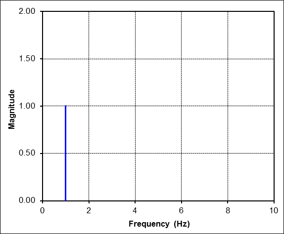
We will work our way up to complex cases by first starting with simple sinusoids. For example, consider this most basic one with amplitude = 1.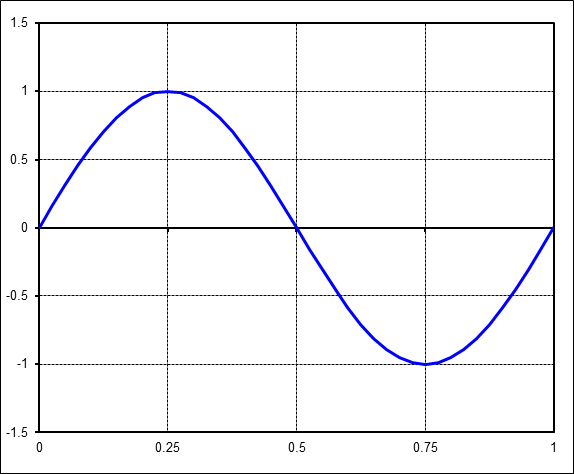
The FFT is simple here. The magnitude is 1 at harmonic 1 on the x-axis. It is at harmonic 1 because the time signal contains exactly 1 complete cycle of a sine wave, neither more nor less.
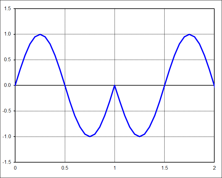
This example shows that the time signal is much more complex this time. It is just busy enough to disguise the underlying harmonics contributing to the plot.
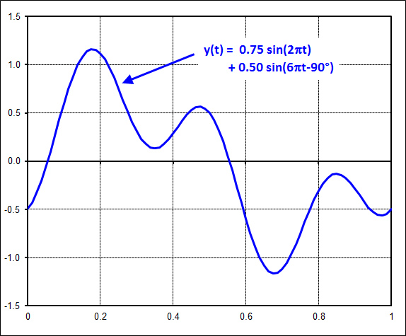
But the FFT is still quite simple. It shows that the complicated time signal is nothing more than the sum of two sine waves. This is the great power of an FFT... to decompose complex time signals into their underlying components.
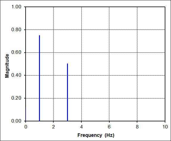
For contrast, consider the time signal below. It is still a nice well-behaved sine function. But the key fact here is that it does not contain an integer number of cycles. It is in fact one and one-quarter cycles.

The FFT of this data is surprisingly complex. There are suddenly many harmonics with energy. This can be very misleading because they suggest (incorrectly) that the signal contains vibrations at 1.0Hz, 2.0Hz, 3.0Hz, etc. But the time signal clearly shows that the 'vibration' was only at 1.25Hz (1 / 0.8sec). The problem here is that the FFT was NOT performed on an integer number of cycles of the time signal!
This is neither right nor wrong. It is simply a fact of life that if you are trying to curve-fit 125% of a sine wave with integer cycles of sine waves, then it will take a lot of them to do so. But again, it doesn't mean that the sine wave in this example contains all these frequencies. It is simply a 1.25Hz signal being curve-fit by 1.0Hz, 2.0Hz, etc sine waves.
Contributions of Individual Harmonics
The table below gives specific results for the first 5 harmonics plotted in the FFT figure just above. The column labeled "\(A_n \cos\)" contains the cosine coefficients, and the column labeled "\(B_n \sin\)" contains the sine coefficients. These are followed by the magnitude and phase lag columns. Recall that the magnitude and phase columns are akin to polar coordinates, while the \(A_n\) and \(B_n\) columns are rectangular in nature.| Freq | \(A_n \cos\) | \(B_n \sin\) | Mag | Phase |
|---|---|---|---|---|
| 0 Hz (DC) | 0.119 | - | 0.119 | - |
| 1 Hz | 0.691 | 0.566 | 0.894 | 39.3° |
| 2 Hz | -0.179 | -0.261 | 0.316 | -124° |
| 3 Hz | -0.069 | -0.128 | 0.145 | -119° |
| 4 Hz | -0.044 | -0.087 | 0.097 | -117° |
| 5 Hz | -0.033 | -0.066 | 0.074 | -116° |
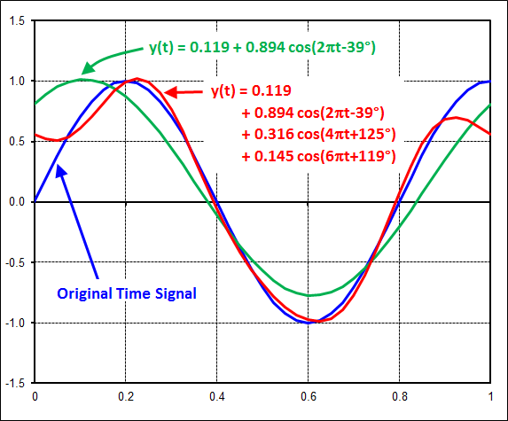
The figure below compares the original time signal (in blue) to the curve-fits containing the first harmonic alone (in green), and the first 3 harmonics (in red). The key thing to note is that the fit improves as more harmonics are added.
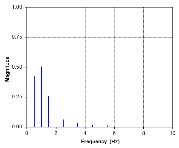
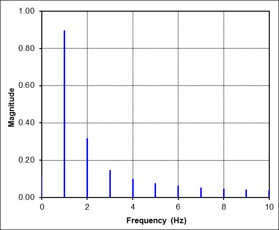
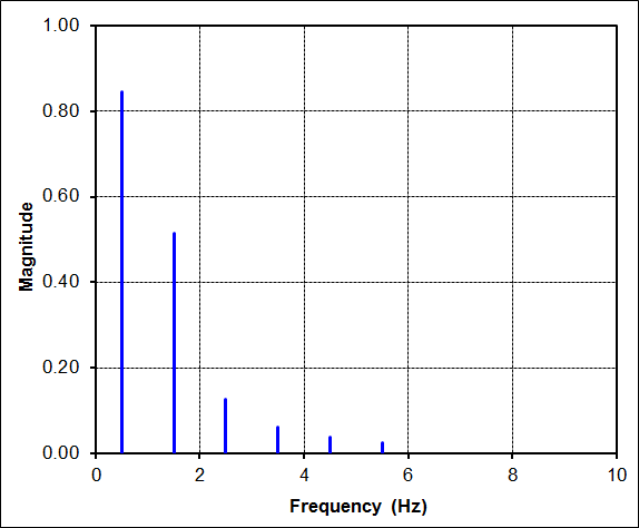
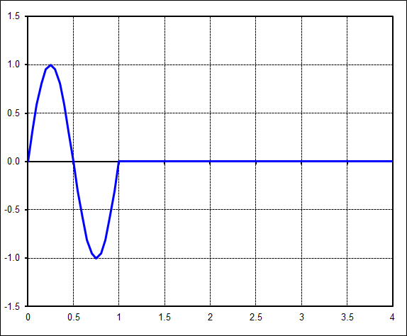
Yet the FFT of this data is also very complex. Again, there are many harmonics with energy. They indicate that the signal contains vibrations at 0.5Hz, 1.0Hz, 1.5Hz, etc. But the time signal clearly shows that the 'vibration' was only at 1Hz, and only for the first second.
The explanation is relatively straight forward, if not obvious. Remember that an FFT is only a regression in which sines and cosines are fit to the time signal. But keep in mind that the sines and cosines being fit are active throughout the whole time window. So this time, since the signal is something (anything) other than a sinusoid over the whole window, then other harmonics must be needed to improve the curve-fit.
And there is another issue in this example, and an important one at that. It is the amplitude of the 1Hz harmonic in the FFT result. It is exactly 1/2 because the time signal has amplitude, 1, but is active for only half of the window. So a conservation of energy requirement is in effect.
In spite of all the harmonics in the FFT result. The only relevant one is at 1Hz, but you must know the time signal in order to know this. You can't tell from the FFT alone.
Contributions of Individual Harmonics
This repeats the above exercise.The table below gives specific results for the first 5 harmonics plotted in the FFT figure just above. The column labeled "\(A_n \cos\)" contains the cosine coefficients, and the column labeled "\(B_n \sin\)" contains the sine coefficients. These are followed by the magnitude and phase lag columns. Recall that the magnitude and phase columns are akin to polar coordinates, while the \(A_n\) and \(B_n\) columns are rectangular in nature.
| Freq | \(A_n \cos\) | \(B_n \sin\) | Mag | Phase |
|---|---|---|---|---|
| 0.0 Hz (DC) | 0.000 | - | 0.119 | - |
| 0.5 Hz | 0.424 | 0.000 | 0.424 | 0° |
| 1.0 Hz | 0.000 | 0.500 | 0.500 | 90° |
| 1.5 Hz | -0.255 | 0.000 | 0.255 | 180° |
| 2.0 Hz | 0.000 | 0.000 | 0.000 | 0° |
| 2.5 Hz | -0.061 | 0.000 | 0.061 | 180° |
The figure below compares the original time signal (in blue) to the curve-fits containing the first harmonic alone (in green), and the first 3 harmonics (in red). The key thing to note is that the fit improves as more harmonics are added.
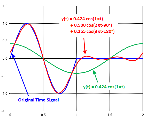
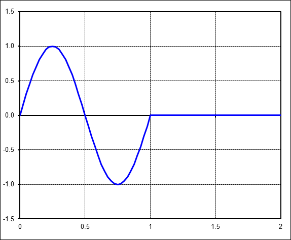
The transform of this signal is also relatively complex, containing several harmonics. But it is clear that the 1Hz, 2Hz, etc harmonics are zero. This is expected because the time signal during the 2nd second will exactly cancel that of the first in the integral transform equations.
Now extend this further. This time, extend the zeroes until the sinusoid is only 1/4 of the total signal.
The FFT result is now as shown below. The important point is that only the harmonic at 1Hz is relevant. All the others only contribute to curve-fitting. Also, the 1Hz amplitude is only 1/4 of the actual time signal amplitude because of the energy conservation effect.
Fourier Transforms of Impulses
Impulse Deformations in a Tire
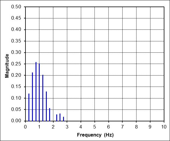
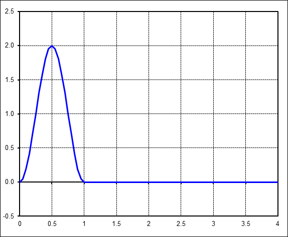
As discussed at the top of this page in the Background Section, the deformations in a tire are not simple sinusoids. They are impulses, so their FFTs are not trivial.Start the sinusoid 90° earlier to make it look like the impulse found in FEA results of rolling tires. Keep the 1/4 ratio as above, although this can in fact be any ratio in a tire: 1/5, 1/6, 1/7, etc. Also, note that although the peak value is 2, the amplitude is still equal to 1.
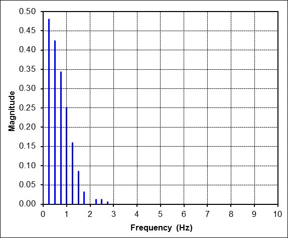
The FFT of this result looks, and is, quite different from the previous FFT. But the amazing result is that the 1Hz component is unchanged. It still has amplitude equal to 1/4 just as before, because, as before, it is the only harmonic that directly matches the frequency of the time pulse. Going in reverse, one would read the amplitude off the FFT at 1Hz and scale it up by a factor of 4 to obtain the amplitude of the actual sine pulse that is present in 1/4 of the total window.
Impact of Pulse Tests on Material Properties
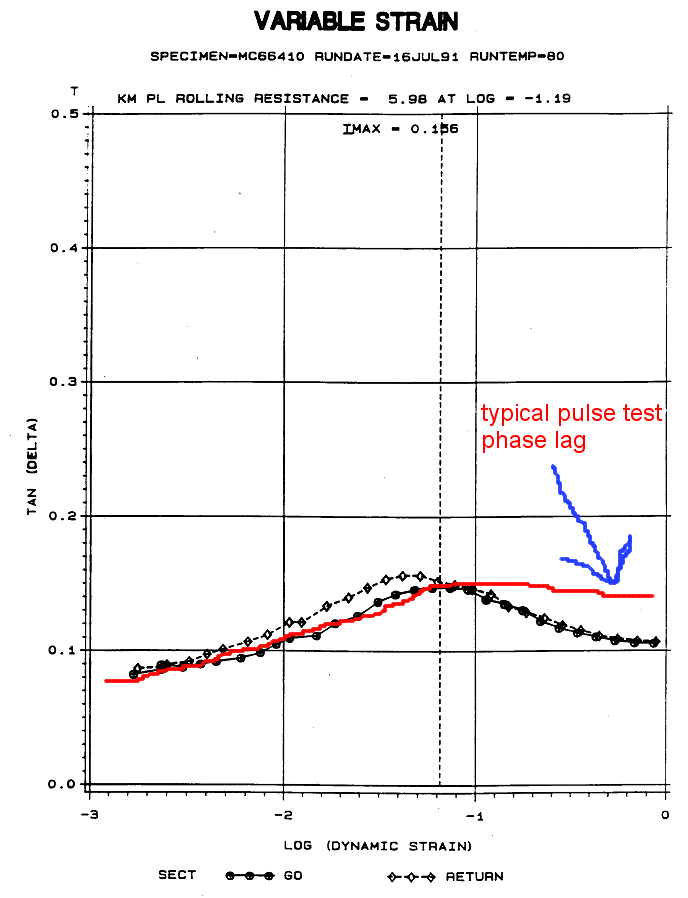
The plot below shows sample time traces of stress and strain signals for a material being subjected to pulse-type lab tests. The time delay between the two is exaggerated for clarity. The phase lag is computed by performing FFTs on both signals and then subtracting the two phase values AT THE SINGLE APPROPRIATE HARMONIC to obtain the phase lag between the stress input and the strain output.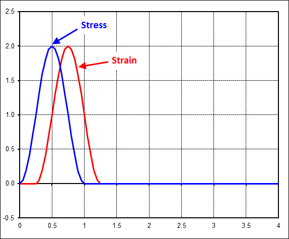
Pulse-type lab tests have a significant impact on the material's phase lag, \(\delta\), at the higher strain levels, above the usual ~8% strain level where \(\tan(\delta)\) usually maxes out under conventional sinusoidal testing. The difference is that under pulse testing, the phase lag follows the red curve in the figure below. (I don't recall any major impact on modulus.)
Synchronization and Transients
Fourier Transforms of Helicopter Data
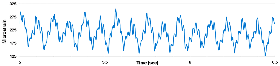
This section presents portions of a briefing on UH-1 "Huey" helicopter vibrations. It addresses one of the major misinterpretations of FFTs, that of assuming vibrations are present at frequencies over which they are not. The full briefing, presented at the 2009 Aging Aircraft Conference, is here.The following graph shows a portion of the vibration signal of the tailboom of a helicopter. It is known that the vibrations occur at 5.39 Hz and multiples of it, as well as 27.65 Hz and multiples of it. The dominant vibration is at
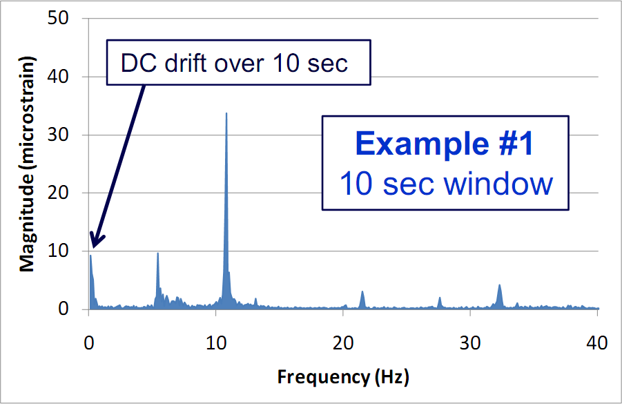
And this graph shows the result of performing an FFT on 10 seconds of the data. It is clear that spikes occur at-and-around the frequencies listed above. But there is also energy present at the lowest frequencies, ~1 Hz. But they do not represent vibrations at these low frequencies, although they are often mistaken for this. They represent transient drifts in the time data over 10 seconds. (As an aside, the frequency spacing is 0.1 Hz because the time window is 10 sec.)
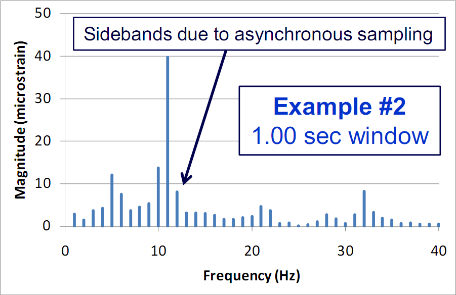
The fact that the data drifts over 10 seconds can be confirmed by instead performing FFTs over shorter time intervals. The following graph shows an FFT of 1 sec of data. The low frequency energy content is now gone. But the sidebands are still present. The frequency spacing is 1 Hz (because the time window is 1 sec), and this is not quite in sync with the 5.39 Hz actual frequency content.
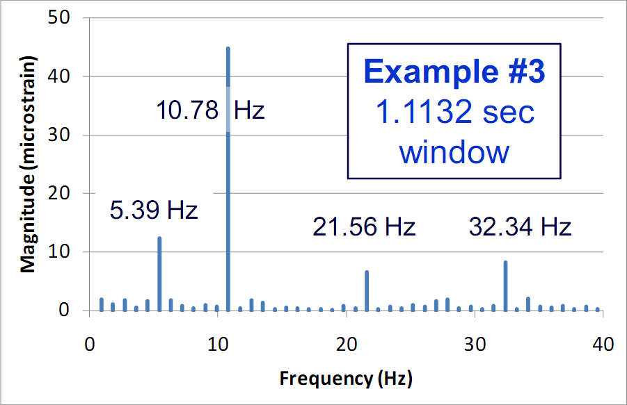
This final graph shows the rather large difference one obtains by simply making a very small change in the time window over which the FFTs are performed. In this case, the time window is 1.1132 sec, which contains exactly six complete cycles of the 5.39 Hz fundamental signal. It is clear that synchronizing the time window over which the FFT is performed with the fundamental vibration frequency has demonstrated that they are "clean". No actual vibrations are present at the sidebands seen in the earlier graph.
The moral of the story here is to synchronize the sampling window with the fundamental vibration frequencies being analyzed. The second key point is to check for transients whenever energy is present at low frequencies. This usually means that the time window is too long.