Introduction
The vast majority of wavelet documents and internet tutorials appear to be written by mathematicians for mathematicians. As a result, they are completely incomprehensible to the rest of us mere mortals, at least in my opinion. The one exception being the book, A Primer on Wavelets and Their Scientific Applications, by James S. Walker, CRC Press, 1999. Without it, I still probably wouldn't understand anything at all about the subject. The chapters are.... Chapter 1, Chapter 2, Chapter 3, and Chapter 4. This webpage is heavily influenced by Chapters 1 and 2.
The story of wavelets began in 1909 with Alfred Haar, who first proposed the 'Haar transform'. But little became of it until 1987 when Ingrid Daubechies demonstrated that general wavelet transforms, of which the Haar transform is a special case, were in fact very useful to digital signal processing. It was at this point that wavelet analysis took off. Nevertheless, wavelets are only about 30 years old and remain much less known or understood by the general tech community than Fourier transforms and moving averages. (Although one could argue that Fourier transforms are still not well understood by a lot of people.)
A major hindrance to wavelet analysis appears to be that there is no easy way to explain how they work. The best approach seems to be a series of examples, with each revealing a new property of the wavelet transform. We will take that approach here.
The Haar Transform
Lets start with an example that demonstrates both signal smoothing and the data compression properties of wavelets using the simplest of wavelet types, the Haar transform. The following example will border on being so simple that it may appear pointless. But be patient. It introduces concepts that will be important later when the analyses are more complex, and much more useful.Consider the following set of eight data points sampled from a signal that tends to be stair-stepped in nature.
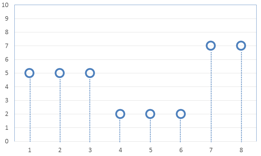
The eight values are
\[ \text{Original 8 values} \quad \rightarrow \quad ( \; 5, \; 5, \; 5, \; 2, \; 2, \; 2, \; 7, \; 7 \; ) \]
Lets call these values: \(y_1, y_2, y_3,\) ...
Now do the following: (i) Pair up the eight data points into four groups of two points each, (ii) and for each pair of values, compute a sum and difference as follows.
\[ \begin{eqnarray} &\text{Sum}_1 & = & y_1 + y_2 = 10 \qquad &\text{Sum}_2 & = & y_3 + y_4 = 7 \qquad &\text{Sum}_3 & = & y_5 + y_6 = 4 \qquad &\text{Sum}_4 & = & y_7 + y_8 = 14 \\ \\ &\text{Diff}_1 & = & y_1 - y_2 = 0 \qquad &\text{Diff}_2 & = & y_3 - y_4 = 3 \qquad &\text{Diff}_3 & = & y_5 - y_6 = 0 \qquad &\text{Diff}_4 & = & y_7 - y_8 = 0 \end{eqnarray} \]
Note - We will later divide these results by \(\sqrt{2}\), but that is not necessary right now since were focusing more on concepts.
It is common to write the sums and differences as
\[ ( \; \text{Sum}_1, \; \text{Sum}_2, \; \text{Sum}_3, \; \text{Sum}_4, \; \text{Diff}_1, \; \text{Diff}_2, \; \text{Diff}_3, \; \text{Diff}_4 \; ) \]
So this looks like
\[ \text{Sums & Diffs} \quad \rightarrow \quad ( \; \underbrace { 10, \; 7, \; 4, \; 14,}_{\text{Sums}} \; \; \underbrace { 0, \; 3, \; 0, \; 0 }_{\text{Diffs}} \, ) \]
We started with eight values, and now we still have eight. Four sums and four differences. This is a kind of conservation of information in that the number of data points remains constant.
Data Compression
Another observation is that we have gotten several zero values for the differences due to the stair-stepped nature of the original data. The data compression capabilities of wavelets comes from the fact that the zero values could be not-stored, thus reducing the file size. And all not-stored numbers would automatically be assumed to equal zero. Since this data tends to be stair-stepped, there could be many zeroes that would not need storing.Inverse Transform
It is easy to go back and recover the original values from the transform. For example, from \(\text{Sum}_1 = 10\) and \(\text{Diff}_1 = 0\), it is easy to get back to \(y_1 = y_2 = 5\) using\[ y_1 = {\text{Sum}_1 + \text{Diff}_1 \over 2} \qquad \text{and} \qquad y_2 = {\text{Sum}_1 - \text{Diff}_1 \over 2} \]
Doing so for all the pairs of numbers gives the original data series again.
Data Smoothing
Now its time to address data smoothing. And in order to do that, first introduce some noise into the data from the above graph.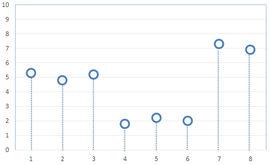
The new noisy values are
\[ \text{8 values with noise} \quad \rightarrow \quad ( \; 5.3, \; 4.8, \; 5.2, \; 1.8, \; 2.2, \; 2.0, \; 7.3, \; 6.9 \; ) \]
The new sums and differences are now
\[ \begin{eqnarray} &\text{Sum}_1 & = & y_1 + y_2 = 10.1 \qquad &\text{Sum}_2 & = & y_3 + y_4 = 7.0 \qquad &\text{Sum}_3 & = & y_5 + y_6 = 4.2 \qquad &\text{Sum}_4 & = & y_7 + y_8 = 14.2 \\ \\ &\text{Diff}_1 & = & y_1 - y_2 = 0.5 \qquad &\text{Diff}_2 & = & y_3 - y_4 = 3.4 \qquad &\text{Diff}_3 & = & y_5 - y_6 = 0.2 \qquad &\text{Diff}_4 & = & y_7 - y_8 = 0.4 \end{eqnarray} \]
And writing as one long list gives
\[ \text{Sums & Diffs of noisy data} \quad \rightarrow \quad ( \; \underbrace { 10.1, \; 7.0, \; 4.2, \; 14.2,}_{\text{Sums}} \; \; \underbrace { 0.5, \; 3.4, \; 0.2, \; 0.4 }_{\text{Diffs}} \, ) \]
Now comes the moment for deep insight! The last 4 difference numbers should be either large values - corresponding to legitimate steps in the original data - or they should be zero. But they should not be the above values of 0.5, 0.2, or 0.4, which are indeed small (relative to other values), but not zero. These small nonzero values indicate that noise is present in the original data.
If the three small non-zero values shouldnt be what they are - what should they be? The answer is they should be 0 if no noise were present. So zero them out!!! This constitutes the data smoothing step.
Zeroing & Data Smoothing
It is very important to understand that the zeroing step here is indeed the data smoothing step!!! This is because an inverse transform is coming up that will now be based on zero-valued differences instead of small-but-nonzero differences.\[ \text{Zeroed-out small diffs} \quad \rightarrow \quad ( \; \underbrace { 10.1, \; 7.0, \; 4.2, \; 14.2,}_{\text{Sums}} \; \; \underbrace { 0.0, \; 3.4, \; 0.0, \; 0.0 }_{\text{Diffs}} \, ) \]
And performing the inverse transform gives
\[ \text{Transformed & smoothed values} \quad \rightarrow \quad ( \; 5.05, \; 5.05, \; 5.2, \; 1.8, \; 2.1, \; 2.1, \; 7.1, \; 7.1 \; ) \]
A graph of the result is here.

Setting the small nonzero differences to zero has smoothed the data. Granted, its not a big deal, and it doesnt look very impressive at this point... But be patient. Better things are coming.
But first, we need to address a few more foundational issues. The first is the idea of energy conservation, which includes that \(\sqrt{2}\) mentioned earlier.
Conservation of Energy
The energy of a data stream is the sum of the squares of the data points. (Sometimes the mean is subtracted out, but we won't do that here.) The energy of the above example containing noise, but before values were zeroed out, is\[ 5.3^2 + 4.8^2 + 5.2^2 + 1.8^2 + 2.2^2 + 2.0^2 + 7.3^2 + 6.9^2 = 191.15 \]
For comparison, compute the energy of the 'sums and differences,' also before values were zeroed out,
\[ 10.1^2 + 7.0^2 + 4.2^2 + 14.2^2 + 0.5^2 + 3.4^2 + 0.2^2 + 0.4^2 = 382.3 \]
which is a different value, obviously. But the amazing thing is that it is exactly twice the energy of the original y-values. Exactly. Therefore, if every sum and difference were instead divided by \(\sqrt{2}\), then the energy of the transformed numbers would be identical to the original energy. In other words, the transform would conserve energy.
Energy Conserving Transforms
Dividing the sum and difference equations through by \(\sqrt{2}\) to make them energy-conserving gives\[ \text{Sum}_1 = {y_1 + y_2 \over \sqrt{2}} \qquad \text{and} \qquad \text{Diff}_1 = {y_1 - y_2 \over \sqrt{2}} \]
It is easy to check that these transformation equations conserve energy because
\[ y_1^2 + y_2^2 \; = \; \text{Sum}_1^2 + \text{Diff}_1^{\,2} \]
And the inverse transform is
\[ y_1 = {\text{Sum}_1 + \text{Diff}_1 \over \sqrt{2}} \qquad \text{and} \qquad y_2 = {\text{Sum}_1 - \text{Diff}_1 \over \sqrt{2}} \]
The presence of the \(\sqrt{2}\) in the equations to ensure energy conservation leads to a very pleasant symmetry of the forward and inverse transforms.
Back to the problem at hand. Dividing the sums and differences through by \(\sqrt{2}\) gives
\[ \text{Sums & Diffs divided by} \sqrt{2} \quad \rightarrow \quad ( \; \underbrace { 7.14, \; 4.95, \; 2.97, \; 10.04,}_{\text{Sums}} \; \; \underbrace { 0.35, \; 2.40, \; 0.14, \; 0.28 }_{\text{Diffs}} \, ) \]
and the energy is now conserved.
\[ 7.14^2 + 4.95^2 + 2.97^2 + 10.04^2 + 0.35^2 + 2.40^2 + 0.14^2 + 0.28^2 \; = \; 191.15 \; = \; 100\% \]
Now that the transform conserves energy, it is possible to quantify the amount of energy removed from the signal when the 3 values were zeroed out. The three values are 0.35, 0.14, and 0.28. Their energy is
\[ 0.35^2 + 0.14^2 + 0.28^2 \; = \; 0.225 \; = \; 0.12\% \]
So the energy of the zeroed-out sums and differences will be \(191.15 - 0.225 = 190.925\), which is still 99.88% of the original signal. Such an energy analysis is a valuable tool for quantifying how much of a signal is removed and how much remains due to the wavelet smoothing process.
The zeroed-out set of sums and differences is now
\[ \text{Zeroed-out small diffs} \quad \rightarrow \quad ( \; \underbrace { 7.14, \; 4.95, \; 2.97, \; 10.04,}_{\text{Sums}} \; \; \underbrace { 0.00, \; 2.40, \; 0.00, \; 0.00 }_{\text{Diffs}} \, ) \]
and their energy is
\[ 7.14^2 + 4.95^2 + 2.97^2 + 10.04^2 + 0.00^2 + 2.40^2 + 0.00^2 + 0.00^2 \; = \; 190.925 \; = \; 99.88\% \]
And the inverse transform is still the exact same result as before because the \(\sqrt{2}\) factors are accounted for.
\[ \text{Transformed values after zeroing small diffs} \quad \rightarrow \quad ( \; 5.05, \; 5.05, \; 5.2, \; 1.8, \; 2.1, \; 2.1, \; 7.1, \; 7.1 \; ) \]
and the energy is
\[ 5.05^2 + 5.05^2 + 5.2^2 + 1.8^2 + 2.1^2 + 2.1^2 + 7.1^2 + 7.1^2 \; = \; 190.925 \; = \; 99.88\% \]
which is the exact same 99.88% value of the earlier zeroed-out sums and differences. As with much of this wavelet introduction so far, the usefulness of the energy and conservation concepts is not yet apparent. But it will become so near the end of the next section on multilevel transforms.
Now that the \(\sqrt{2}\) has been incorporated into the process, it is a full-fledged 1-level, 2-point, wavelet transform that conserves energy. This simple initial case was actually first discovered (developed?) by Alfred Haar in 1909 and is called the Haar Transform. It is now considered to be the first application of wavelets, even though the name wavelet, and other applications of them, didnt come along until much later.
Finally, we have so far only performed a 1-level transform because we only computed sums and differences once. Higher level transforms are possible. The next section describes how they work.
Multilevel Transforms
Go back to the transformed data with the \(\sqrt{2}\) incorporated, but before the small values were zeroed out.\[ \text{Sums & Diffs divided by} \sqrt{2} \quad \rightarrow \quad ( \; \underbrace { 7.14, \; 4.95, \; 2.97, \; 10.04,}_{\text{1st Sums}} \; \; \underbrace { 0.35, \; 2.40, \; 0.14, \; 0.28 }_{\text{1st Diffs}} \, ) \]
The process for doing a 2-level transform is to simply repeat the sum and difference operations on the first four sums again. The four difference terms (the "1st diffs") are not touched.
\[ \text{Sums:} \quad {7.14 + 4.95 \over \sqrt{2}} = 8.55 \quad {2.97 + 10.04 \over \sqrt{2}} = 9.20 \qquad \text{Diffs:} \quad {7.14 - 4.95 \over \sqrt{2}} = 1.55 \quad {2.97 - 10.04 \over \sqrt{2}} = -5.00 \]
Replacing the "1st Sums" with the two new sums and differences now gives
\[ \text{2-Level sums and diffs} \quad \rightarrow \quad ( \; \underbrace { 8.55, \; 9.20, }_{\text{2nd Sums}} \; \; \underbrace { 1.55, \; -5.00, }_{\text{2nd Diffs}} \; \; \underbrace { 0.35, \; 2.40, \; 0.14, \; 0.28 }_{\text{1st Diffs}} \, ) \]
And a third and final transform can be performed on the final two sums, this time leaving the 1st and 2nd differences untouched. This gives
\[ \text{3-Level sums and diffs} \quad \rightarrow \quad ( \; \underbrace {12.55, }_{\text{3rd Sum}} \; \; \underbrace {-0.46, }_{\text{3rd Diff}} \; \; \underbrace { 1.55, \; -5.00, }_{\text{2nd Diffs}} \; \; \underbrace { 0.35, \; 2.40, \; 0.14, \; 0.28 }_{\text{1st Diffs}} \, ) \]
This is a 3-level 2-point wavelet transform. The first value is a sum, and all the other values are differences, and all values become candidates to be zeroed out. Furthermore, the entire process conserves energy.
\[ 12.55^2 + 0.46^2 + 1.55^2 + 5.00^2 + 0.35^2 + 2.40^2 + 0.14^2 + 0.28^2 \; = \; 191.15 \; = \; 100\% \]
The importance of conserving energy can now be seen because it means that a single threshold value can be selected, below which values are zeroed out, and applied to the 1st, 2nd, and 3rd differences without fear of bias. Had the transforms not been energy-conserving, then it would not be clear as to what effect a given threshold level would have on the three different difference steps. (And no, it is not absolutely necessary to apply the same threshold level to all difference sets.)
Number of Data Points & Powers of 2
It is time to stress that all these transforms require an even number of data points, otherwise, computing complete sets of sums and differences would be impossible. Even the 1st set of sums and differences would be impossible if the number of data points were odd.There are multiple ways of overcoming this. If the number of points is odd, then any data point could be duplicated to obtain an even number. Or alternatively, a spline interpolation routine could be implemented to obtain an even number. The possibilities are endless.
However, if multilevel transforms are desired, and they usually are, restrictions on the number of data points grow. It should be clear from the example here that the desired number of points is a power of 2, just as with Fast Fourier Transforms (FFTs). Once again, a spline routine is probably the best way to interpolate the raw data into a new set with the desired number of points.
And finally, though not yet obvious, the data points really should be equally spaced in time or position. This is another property in common with FFTs. The wavelet transform and the FFT are both fed only y-values and therefore never see the x (or time) values to determine if the y-values are equally spaced. They are just assumed to be. If not, then although the transforms will still run, the quality of the results will be diminished.
Vector-Based Notation
First, define the following vector.
\[ \vec{\bf{v}} = \left({1 \over \sqrt{2}}, {1 \over \sqrt{2}}\right) \]
And recognize that the sum transforms can be performed as follows.
\[ \begin{array} \, \text{Sum}_1 = \vec{\bf{v}} \cdot (y1, \; y2) = {1 \over \sqrt{2}} \: y_1 + {1 \over \sqrt{2}} \: y_2 \\ \\ \text{Sum}_2 = \vec{\bf{v}} \cdot (y3, \; y4) = {1 \over \sqrt{2}} \: y_3 + {1 \over \sqrt{2}} \: y_4 \end{array} \]
Then define a second vector for the difference operations.
\[ \vec{\bf{w}} = \left({1 \over \sqrt{2}}, -{1 \over \sqrt{2}}\right) \]
The difference transforms can now be written as
\[ \begin{array} \, \text{Diff}_1 = \vec{\bf{w}} \cdot (y1, \; y2) = {1 \over \sqrt{2}} \: y_1 - {1 \over \sqrt{2}} \: y_2 \\ \\ \text{Diff}_2 = \vec{\bf{w}} \cdot (y3, \; y4) = {1 \over \sqrt{2}} \: y_3 - {1 \over \sqrt{2}} \: y_4 \end{array} \]
The \(\vec{\bf{w}}\) vector is called the wavelet because it waves around zero, having equal parts above and below it. In fact
\[ w_1 + w_2 \; = \; 0 \]
Clearly, both \(\vec{\bf{v}}\) and \(\vec{\bf{w}}\) are unit vectors because
\[ w_1^2 + w_2^2 \; = \; v_1^2 + v_2^2 \; = \; 1 \]
And finally, \(\vec{\bf{v}}\) and \(\vec{\bf{w}}\) are orthogonal because
\[ \vec{\bf{v}} \cdot \vec{\bf{w}} \; = \; \left({1 \over \sqrt{2}}\right) \! \left({1 \over \sqrt{2}}\right) - \left({1 \over \sqrt{2}}\right) \! \left({1 \over \sqrt{2}}\right) \; = \; 0 \]
Inverse Transforms
The inverse transform is also simple to express as vector operations. Assume we had stopped after the first 1-level forward transform above, the one that gave us four sums and four differences. It is just a matter of multiplying those sums and differences by the \(\vec{\bf{v}}\) and \(\vec{\bf{w}}\) vectors again to get back, though not as dot products this time. The process contains 3 steps.- First, create a sum vector as follows
\[ \text{Sum Vector} \quad \rightarrow \quad ( \; \text{Sum}_1 * \vec{\bf{v}}, \; \text{Sum}_2 * \vec{\bf{v}}, \; \text{Sum}_3 * \vec{\bf{v}}, \; \text{Sum}_4 * \vec{\bf{v}} \; ) \]
Note this is actually 8 separate values because each ( \(\text{Sum} * \vec{\bf{v}}\) ) term is a scalar multiplied by a 2-D vector, creating a 2-valued result. The * means to simply multiply the scalar value throughout the vector, nothing more. The 8 individual terms are
\[ \text{Sum Vector} \quad \rightarrow \quad (\; \text{Sum}_1 * v_1, \; \text{Sum}_1 * v_2, \; \text{Sum}_2 * v_1, \; \text{Sum}_2 * v_2, \; \text{Sum}_3 * v_1, \; \text{Sum}_3 * v_2, \; \text{Sum}_4 * v_1, \; \text{Sum}_4 * v_2 \; ) \]
-
Next, create a "diff vector as follows
\[ \text{Diff vector} \quad \rightarrow \quad ( \; \text{Diff}_1 * \vec{\bf{w}}, \; \text{Diff}_2 * \vec{\bf{w}}, \; \text{Diff}_3 * \vec{\bf{w}}, \; \text{Diff}_4 * \vec{\bf{w}} \; ) \]
This is also 8 terms instead of 4, just like the Sum result above. The 8 individual terms are
\[ \text{Diff Vector} \quad \rightarrow \quad (\; \text{Diff}_1 * w_1, \; \text{Diff}_1 * w_2, \; \text{Diff}_2 * w_1, \; \text{Diff}_2 * w_2, \; \text{Diff}_3 * w_1, \; \text{Diff}_3 * w_2, \; \text{Diff}_4 * w_1, \; \text{Diff}_4 * w_2 \; ) \]
-
Finally add the sum and diff vectors together, term by term, and youre done.
The vector-based transform process presented here applies regardless of how complex the wavelet transforms become.
Real World Example
This example demonstrates the usefulness of the Haar transform in a real world situation. The graph below shows some raw data, which is clearly stair stepped, and also contains a fair amount of noise. The objective is to smooth out the noise. And the goal is to do so without rounding off the corners of the data as would happen if moving averages were applied.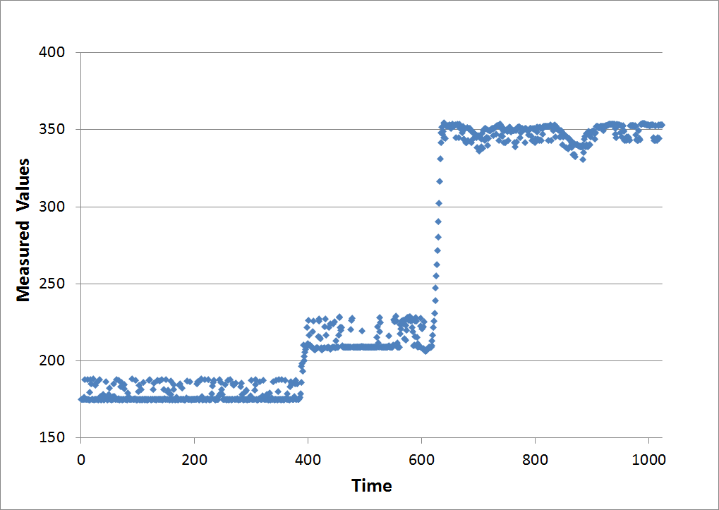
This graph shows the transformed result. Ten levels of transformation were applied to the 1024 data points, so that the 1st value is the only sum, and all other values are differences. Note that several values do exceed '100'. Nevertheless, the graph is zoomed-in to better show the many smaller values.

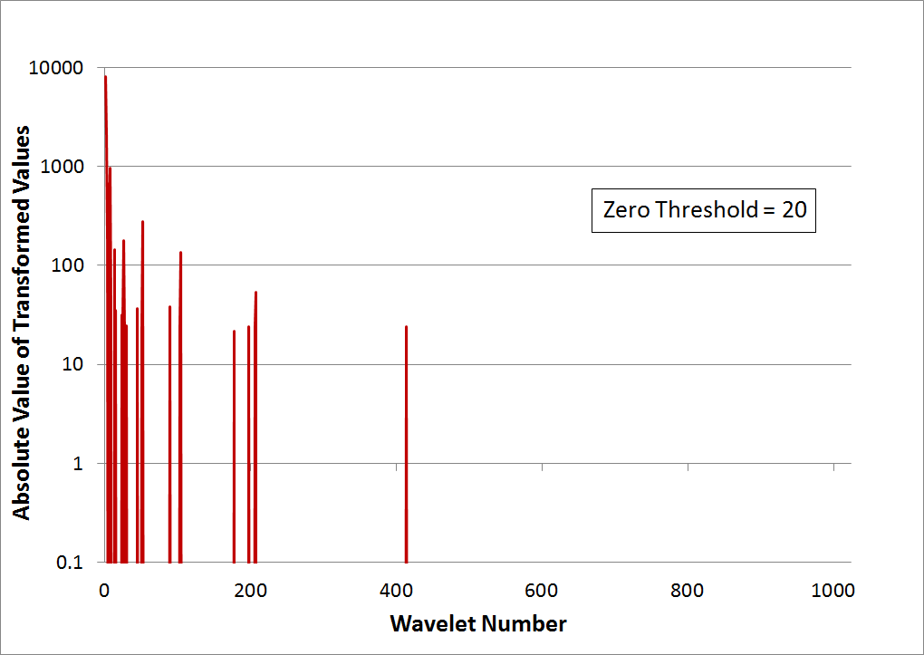
Though not necessary, an additional analysis step is shown in the graph below. It consists of first taking the absolute value of all the transformed results, and then plotting them on a log scale. The advantage is that the noise floor becomes easy to identify. In this case, it is approximately 10.

The graph below shows that a rather aggressive value of '20' has been chosen as the threshold and all points with absolute values below this have been zeroed out. Although many points were eliminated, only 0.36% of the signal's energy has been removed. 99.6% remains even though about 98% of the values have been zeroed out, leaving only 2% of the original number of nonzero values. This once again demonstrates the great data compression capabilities of wavelets.
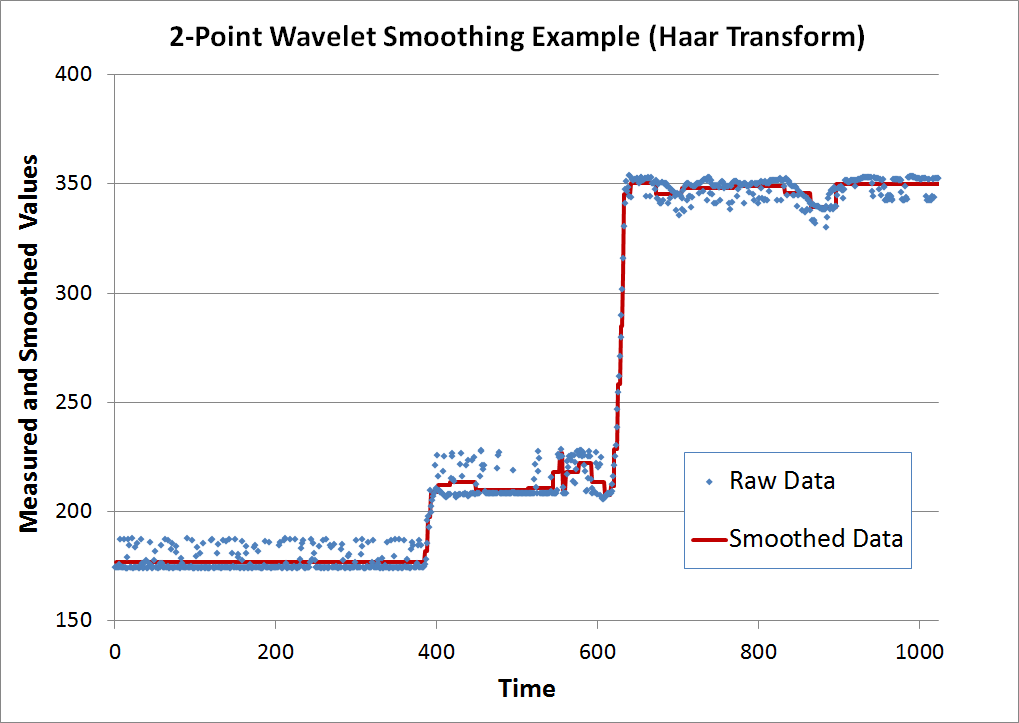
The final graph shows the inverse transform result and the original data for comparison. The result possesses three desirable properties. First, it minimizes random oscillations. In fact, it comes close to eliminating them completely. Second, it does not round-off corners by under or over-shooting when steps occur at time = 400 and time = 600. Third, it accomplishes this with only 2% of the original number of nonzero values, a 98% effective compression ratio.
Daubechies Wavelets
The next sections will extend the \(\vec{\bf{v}}\) and \(\vec{\bf{w}}\) vectors to higher orders: 4, 6, 8, etc points. (Daubechies Wavelets don't come in odd lengths.) So what is the point of using vectors of longer lengths? The amazing answer is that they will prove to be able to smooth functions that are linear, quadratic, cubic, etc.
4-Point Daubechies Wavelets
The 4-point vectors are\[ \begin{eqnarray} \vec{\bf{v}} & = & ( \;\;\;0.4829629, \;\;\;\; 0.8365163, \;\;\; 0.2241439, \; -0.1294095 \; ) \\ \\ \vec{\bf{w}} & = & ( \; -0.1294095, \; -0.2241439, \;\;\; 0.8365163, \; -0.4829629 \; ) \end{eqnarray} \]
The 4-point wavelets retain all the same properties as the 2-point Haar wavelets.
\[ \begin{eqnarray} \sum v_i = \sqrt{2} \qquad \qquad \qquad \qquad \sum w_i = 0 \\ \\ \sum v_i^2 = 1 \qquad \qquad \qquad \qquad \sum w_i^2 = 1 \\ \\ \vec{\bf{v}} \cdot \vec{\bf{w}} = 0 \qquad \qquad \qquad \end{eqnarray} \]
And there is an additional property in common with Haar transforms that was not mentioned earlier. It is the relationship between components of the \(\vec{\bf{v}}\) and \(\vec{\bf{w}}\) vectors.
\[ w_1 = v_4 \qquad w_2 = -v_3 \qquad w_3 = v_2 \qquad w_4 = -v_1 \]
It is part of the larger, more general relationship, which is
\[ w_1 = v_N \qquad w_2 = -v_{N-1} \qquad w_3 = v_{N-2} \qquad w_4 = -v_{N-3} \;\; \text{...} \]
where \(N\) is the number of vector components: 2, 4, 6, etc.
This relationship extends to all Daubechies wavelet transforms, regardless of order, and was true of the Haar transform as well.
HOWEVER! The 4-point wavelet vector, \(\vec{\bf{w}}\), also has one additional remarkable property that its 2-point cousin does not. It is this
\[ 1 * w_1 + 2 * w_2 + 3 * w_3 + 4 * w_4 = 0 \]
This can be written as
\[ \vec{\bf{y}} \cdot \vec{\bf{w}} = 0 \]
where \(\vec{\bf{y}} = (1, 2, 3, 4)\) is the measured data being smoothed. It in fact works for any linear vector, such as \((10, 20, 30, 40)\), or \((2, 4, 6, 8)\), or even \((5, 4, 3, 2)\). This is relevant to data compression because linear functions will produce zero wavelet transform components, which do not need to be stored.
4-Point Wavelet Transform of Linear Data
Start with the following eight values, which obviously increase linearly.\[ \text{Original 8 values} \quad \rightarrow \quad (\;1,\;2,\;3,\;4,\;5,\;6,\;7,\;8\;) \]
The first level 4-point transform of this gives
\[ \text{1st Sums & Diffs} \quad \rightarrow \quad ( \; \underbrace { 2.31,\;5.14,\;7.97,\;10.04, }_{\text{1st Sums}} \; \; \underbrace { 0,\;\;0,\;\;0,\; -2.83 }_{\text{1st Diffs}} \, ) \]
Several zeroes result from the dot products, \(\vec{\bf{y}} \cdot \vec{\bf{w}}\), for the subsets of \(\vec{\bf{y}}\).
\[ \vec{\bf{y}} = (\,1,\;2,\;3,\;4\,) \qquad \quad \vec{\bf{y}} = (\,3,\;4,\;5,\;6\,) \qquad \quad \vec{\bf{y}} = (\,5,\;6,\;7,\;8\,) \]
The last value, -2.83, merits special attention. It is the result of the dot product, \(\vec{\bf{y}} \cdot \vec{\bf{w}}\), when \(\vec{\bf{y}} = (7,\;8,\;1,\;2)\). Yes, the values "wrap around"! Clearly, \(\vec{\bf{y}} = (7,\;8,\;1,\;2)\) is not a linear vector and this is why the -2.83 result is not zero.
Performing the second level transform gives
\[ \text{2nd Sums & Diffs} \quad \rightarrow \quad ( \; \underbrace { 5.90, \; 12.10, }_{\text{2nd Sums}} \; \; \underbrace { 0.37, \; -3.83, }_{\text{2nd Diffs}} \; \; \underbrace { 0,\;\;0,\;\;0,\; -2.83 }_{\text{1st Diffs}} \, ) \]
And the third transform gives
\[ \text{3rd Sums & Diffs} \quad \rightarrow \quad ( \; \underbrace {12.73, }_{\text{3rd Sum}} \; \; \underbrace {-4.38, }_{\text{3rd Diff}} \; \; \underbrace { 0.37, \; -3.83, }_{\text{2nd Diffs}} \; \; \underbrace { 0,\;\;0,\;\;0,\; -2.83 }_{\text{1st Diffs}} \, ) \]
Three of the eight values are now zero. This demonstrates the natural ability of 4-point wavelet transforms to reduce the amount of data requiring storage (by not storing zeroes) when the data is linearly increasing, or decreasing.
This also impacts data smoothing because now, a 4-point wavelet transform can be applied to noisy data that contains ramps, not just stair-steps as was the case for 2-point Haar transforms.
4-Point Wavelet Smoothing of Noisy Data
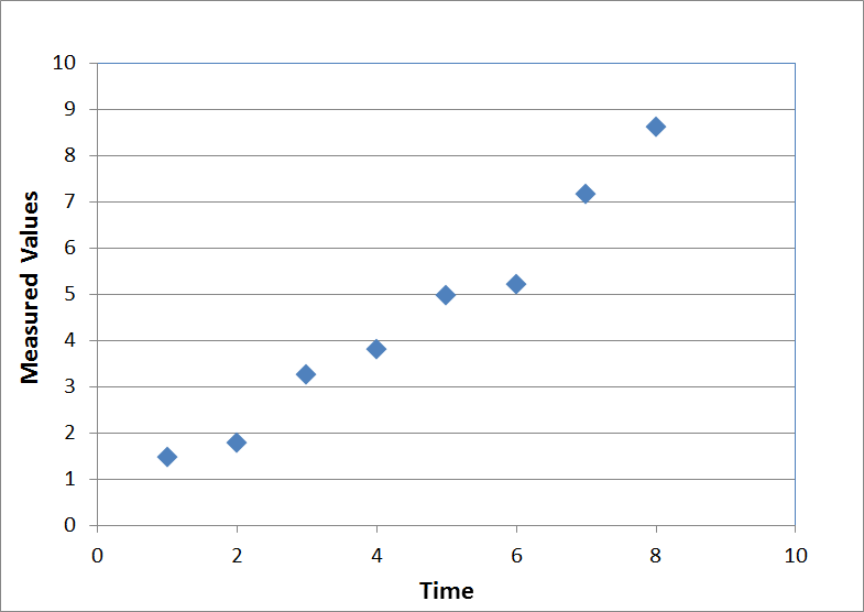
Suppose the data did contain noise, and instead of being 1, 2, 3, 4, etc, the values were instead\[ \text{8 values with noise} \quad \rightarrow \quad (\;1.47,\;1.77,\;3.24,\;3.79,\;4.96,\;5.20,\;7.16,\;8.62\;) \]
A graph of these (noisy) values is shown here
The transformed values are
\[ \text{Transformed values} \quad \rightarrow \quad (\;12.80,\;-4.70,\;-0.62,\;-3.82,\;\;0.29,\;\;0.37,\;\;0.02,\;-2.48\;) \]
And after zeroing out the three values below 0.4, and inverse-transforming back, we get the following
\[ \text{Smoothed values} \quad \rightarrow \quad (\;1.41,\;1.82,\;2.96,\;3.91,\;4.88,\;5.84,\;7.11,\;8.31\;) \]
which are plotted here.

The red points do not form a perfectly straight line because they are not supposed to. Remember, this is not a linear regression. It is still a type of moving average, just a very powerful one. Regardless, the smoothed red points certainly contain less noise than the raw data (blue points).
Higher Order Daubechies Wavelets
To review... the 2-point transform was suited to functions with constant values, and the 4-point transform was suited to linear functions. The next step is 6-point transforms that turn out to be ideal for quadratic functions. (And 8-pointers will go with cubic functions, and so on.)The 6-point values are
\[ \begin{eqnarray} \vec{\bf{v}} & = & (\;0.33267055,\;\;0.80689151,\;\;\;\;0.45987750,\;-0.13501102,\;-0.08544127,\;\;\;\;0.03522629\;) \\ \\ \vec{\bf{w}} & = & (\;0.03522629,\;\;0.08544127,\;-0.13501102,\;-0.45987750,\;\;\;\;0.80689151,\;-0.33267055\;) \end{eqnarray} \]
The 6-point wavelets possess all the properties of their 2-point and 4-point cousins, including
\[ 1 * w_1 + 2 * w_2 + 3 * w_3 + 4 * w_4 + 5 * w_5 + 6 * w_6 = 0 \]
which is just the 6-point version of the same linear property possessed by the 4-point transform. However, the 6-point wavelet provides an additional new property
\[ 1^2 * w_1 + 2^2 * w_2 + 3^2 * w_3 + 4^2 * w_4 + 5^2 * w_5 + 6^2 * w_6 = 0 \]
This is the ability to transform quadratic functions into zero-valued wavelet coefficients. So for the first time now, wavelet transforms can be applied to functions with curvature, not just stair-steps and linear ramps, in order to perform data compression and smoothing.
Likewise, an 8-point wavelet transform is suited to smoothing cubic data. And on and on. In general, the relationship between the order of the wavelet, \(N\), and the exponential power of the data smoothing, e.g., linear, quadratic, etc, is \(N/2-1\).
A long list of \(\vec{\bf{v}}\) values for higher order wavelets can be found here. It cannot be called complete or exhaustive because there are, in fact, an infinite number of wavelet transforms of ever increasing numbers of points. Nevertheless, the list is certainly 'enough'.
Fourier Transforms
Part of me hates to go here because too many other people already spend too much time trying to introduce wavelets by instead talking about Fourier transforms (FFTs). They yield to the temptation of justifying wavelets by pointing out the weaknesses of FFTs. But when I read such articles, I find that although I'm learning a lot about FFT weaknesses, I'm still not learning anything about wavelets. So I will not be harping much on FFTs here. Instead, I want to point out some of their positive aspects that we take for granted, and in the process, set the stage for the next topic of discussion on wavelets. Here goes...Consider all the things that come to mind when you see the graph below representing a Fourier transform.

- The signal is primarily a single sine wave at a medium frequency, not too high and not too low.
- There is a small amount of white noise present in the signal, as evidenced by the small values all across the frequency range.
- An inverse transform would produce a sine wave with random noise riding on top.
- Zeroing out the white noise before transforming would produce a nice clean sine wave.
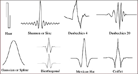
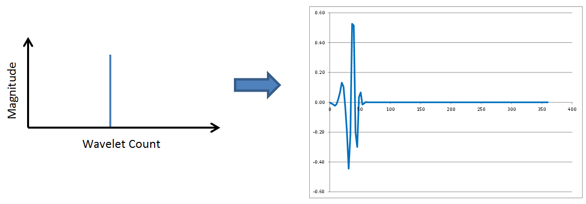
Fundamental Wavelet Shapes
Wavelets have fundamental shapes similar in concept to the fact that FFTs have fundamental shapes involving of sines and cosines. It turns out the fundamental shape of a wavelet depends on the number of points (2, 4, 6, etc) involved in the transform. The way to see this is to start with a single spike in transformed space, as shown here, and perform inverse wavelet transforms on it with different numbers of wavelet points.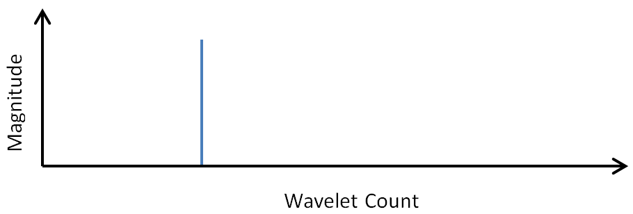
Here are the results of 2, 4, 6, 8, and 10 point inverse wavelet transforms on the spectrum shown above.
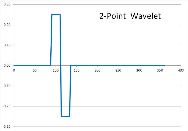
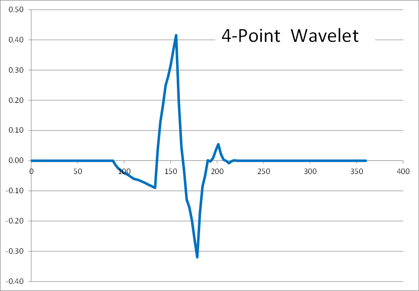
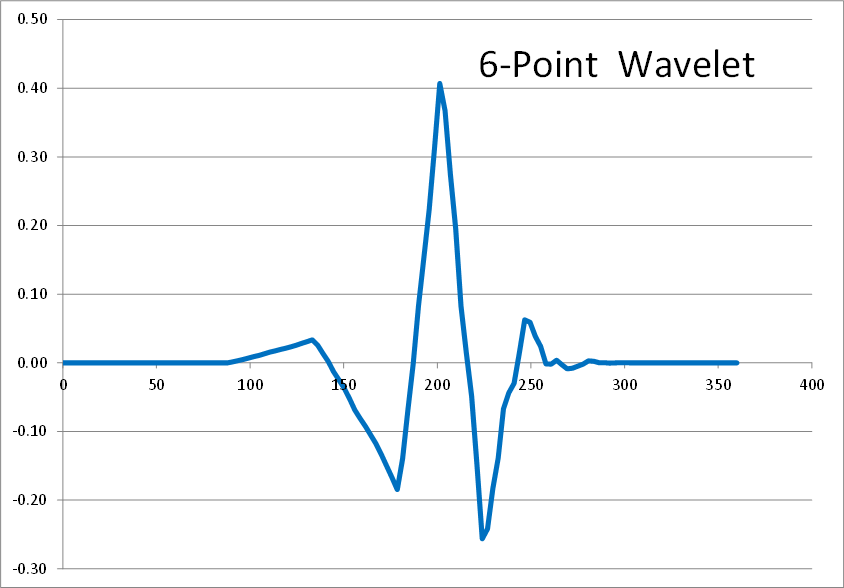
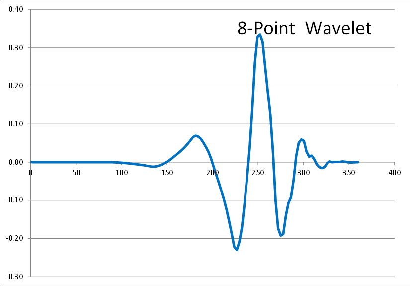

All of these results come from the same single-spiked wavelet spectrum above. But the results are clearly quite different depending on how many points are used in the wavelet. The 2-point wavelet (Haar Transform) still looks stair-stepped as expected. The 4-point result looks like a shark fin, or rose bush thorn. The 6-point result looks like a series of straight lines. And the 8-point and higher results finally get rid of sharp corners and start to resemble short portions of sine waves.
So the number of points in a wavelet transform can be chosen depending on what kind of data you are working with. If it is stair-stepped, go with the 2-point Haar transform. If it is smooth and curvy, go with at least 8 points.
Data Smoothing Example
Here's is a 2nd real world example of using wavelets to smooth noisy data. The blue dots are strain predictions of a transient nonlinear finite element analysis (FEA). The result is not quite converged, and therefore appears noisy. The goal is to smooth the data by performing a wavelet transform, zeroing out the noise, and then inverse transforming to get back to a smooth signal (shown in red). Here are the results of using 2, 4, 6, 8, and 10 points in the wavelet transform.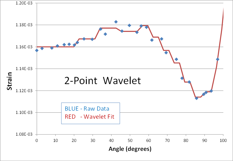
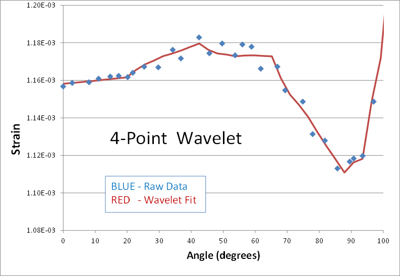
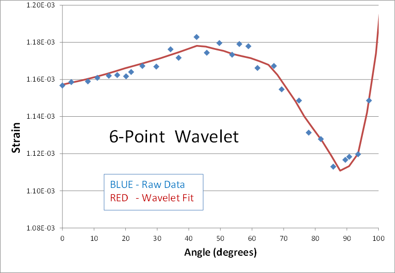
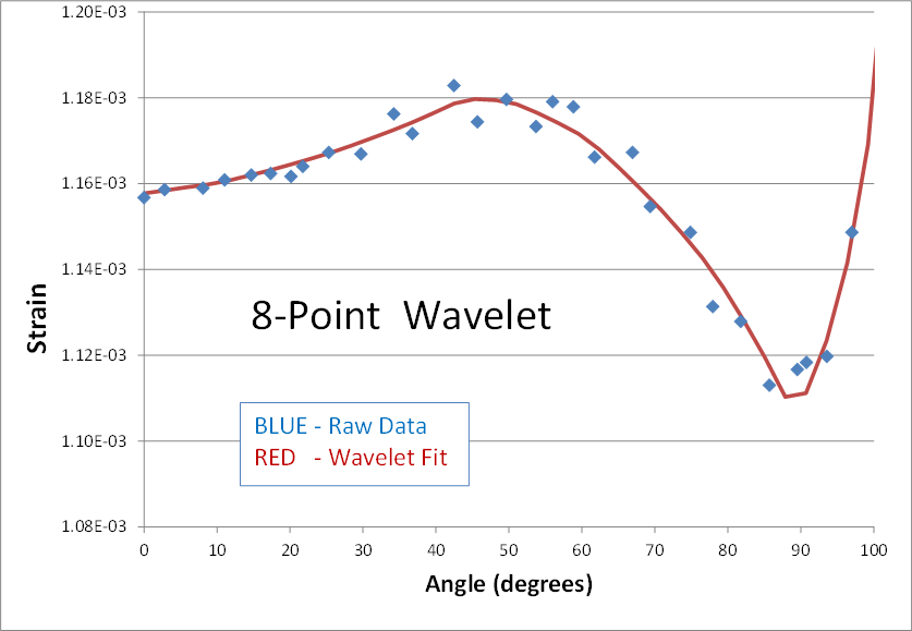

The blue data points have been smoothed in each case, but the personality of the n-point wavelet is still present each time. The 2-point result continues its digital theme. It might be good for processing digital electronics signals. The 4-point result still looks like shark fins. (I cant imagine why anyone would ever need this one.) The 6-point result looks faceted in nature... a collection of straight lines. And its not until the 8 and 10-point transforms that curvy results are obtained.
This example starts to highlight the advantages of wavelets over moving averages, and even Fourier Transforms, when it comes to smoothing data. The only adjustable parameter in a moving average is the number of smoothed points. An FFT can only fit sine waves to the data. In contrast, wavelets provide many more adjustable parameters to optimize the data smoothing process for the task at hand.
Frequency Content of Wavelets
It turns out wavelets have frequency content analogous to Fourier transforms. Compare the following 8-point inverse transforms and note how the period of each wavelet decreases (its frequency increases) on the right side of the figure as the spike in the spectrum moves to the right.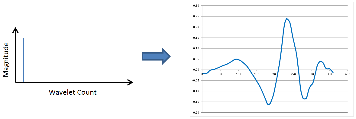
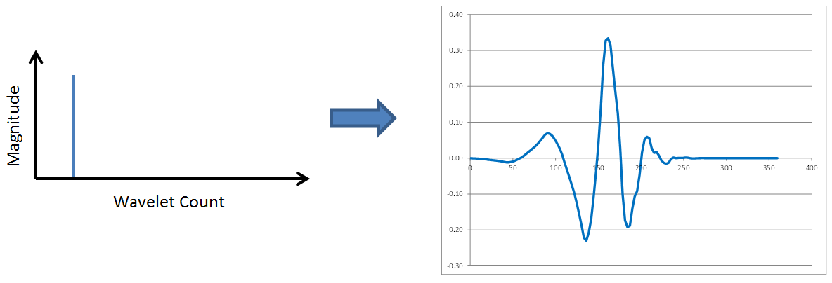
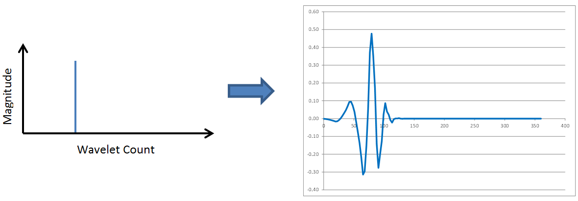
No surprises so far. Wavelet transforms possess the same frequency content properties, low to medium to high frequencies, as Fourier transforms. However, check out the following two figures in which the spike continues to move to the right.
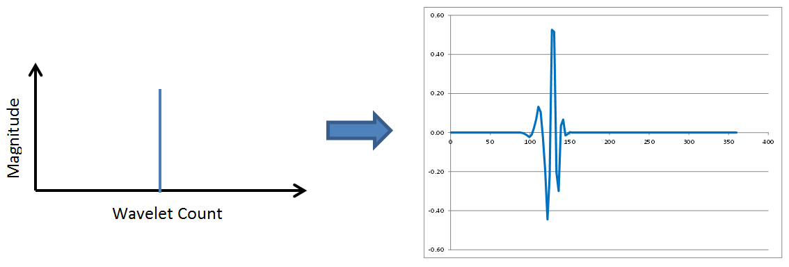

This time, the frequency content has not changed at all. But the position of the wavelet within the overall signal has moved to the right as the spike in the wavelet spectrum moves right. The revelation here is that wavelets contain both frequency and location information. This is a new and different concept that is completely absent in Fourier transforms. FFTs correspond to sinusoids that each extend throughout the entirety of a data window. Not so with wavelets. Wavelets report on WHAT frequencies are present in the data, and WHEN in the time window they occur.
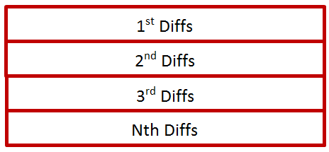
This is a consequence of the wavelet transform algorithm. Recall how the sums and differences are first computed and stored in the 1st and 2nd half of the data. Then this is done again on the 1st and 2nd quarter, then eighths, etc. Graphically, the process looks like this.
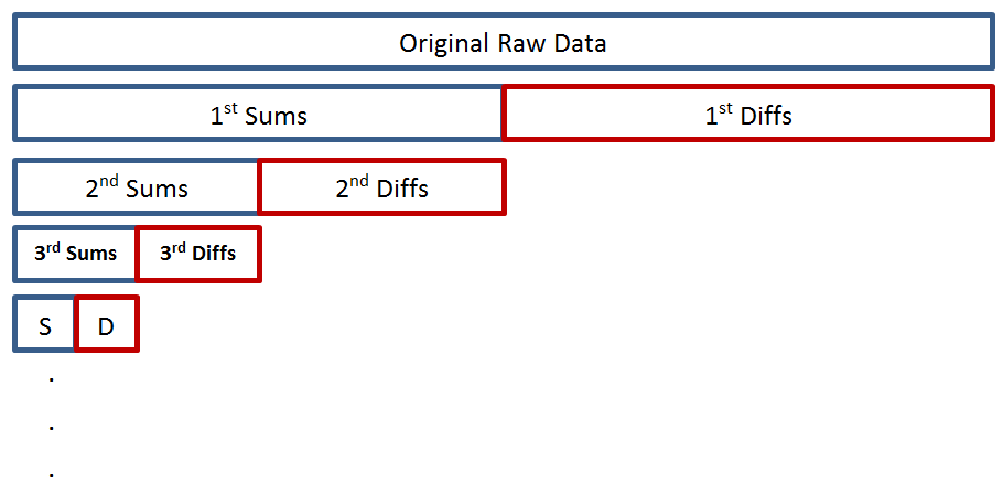
This is all stored over the original raw data as

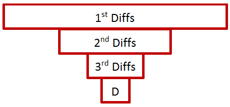
It turns out that all values within a Diff-Box correspond to the same frequency, and their position within the box corresponds to the location of where that frequency is present in the overall signal. The 1st diffs are the highest frequencies. The 2nd diffs are the second highest. And so on.
In the end, the first data point will be the only sum, the 2nd point will be the 1st harmonic, the 3rd and 4th points will function like 2nd harmonics and distinguish position according to the 1st or 2nd half of the original data, the 5th 8th points will function like 4th harmonics (nope, no 3rd harmonic) and also distinguish in which quarter of the original data the particular frequency is present, and the 9th 16th points will act like 8th harmonics, and on and on. Note finally that the frequency content doubles rather than increases by 1 each time. This makes wavelets ideal for music, auditory, vibration comfort, etc analyses involving human response.
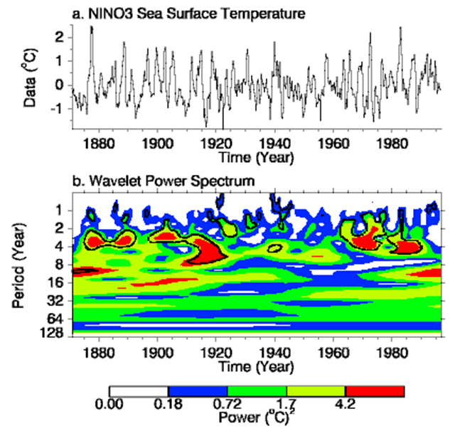
Finally, it is possible to stack the results up in a type of carpet plot as follows.
And then stretch them out. This puts the highest frequencies at the top and the lowest frequencies at the bottom.
An example of this that floats around the internet is a carpet plot of temperatures due to El Nino over the last 100+ years. It shows that the largest temperature oscillations have wavelengths of 4 yrs and occur around 1915. Such an interpretation of the data would be impossible with FFTs.