Introduction
The von Mises stress is often used in determining whether an isotropic and ductile metal will yield when subjected to a complex loading condition. This is accomplished by calculating the von Mises stress and comparing it to the material's yield stress, which constitutes the von Mises Yield Criterion.
The objective is to develop a yield criterion for ductile metals that works for any complex 3-D loading condition, regardless of the mix of normal and shear stresses. The von Mises stress does this by boiling the complex stress state down into a single scalar number that is compared to a metal's yield strength, also a single scalar numerical value determined from a uniaxial tension test (because that's the easiest) on the material in a lab.
It should be noted that this is not an exact science like, say \(F = m\,a\). It is an empirical process, with inherent error and deviations. In fact, there is no hard & fast rule saying that metals must yield according to von Mises yield criteria. It is as much a coincidence as anything. Nevertheless, it does work very well and remains the method of choice a full century after it was first proposed.
History
In 1931, Taylor and Quinney [4] published results of tests on copper, aluminum, and mild steel demonstrating that the von Mises stress is a more accurate predictor of the onset of metal yielding than the maximum shear stress criterion, which had been proposed by Tresca [5] in 1864 and was the best predictor of metal yielding to date. Today, the von Mises stress is sometimes referred to as the Huber-Mises stress in recognition of Huber's contribution to its development. It is also called Mises effective stress and simply effective stress.
Technical Background
A complete understanding of the von Mises stress requires an understanding of hydrostatic and deviatoric components of stress and strain tensors, Hooke's Law, and strain energy density. The hydrostatic and deviatoric stresses and strains have already been reviewed. And Hooke's Law has already been touched on here and here, but will need to be discussed in additional detail on this page as well. Strain energy density will also be introduced here.Hydrostatic and Deviatoric Components
Recall that any stress tensor can be decomposed into the sum of hydrostatic and deviatoric stresses as follows\[ \sigma_{ij} = {1 \over 3} \delta_{ij} \sigma_{kk} + \sigma'\!_{ij} \]
where \( {1 \over 3} \delta_{ij} \sigma_{kk} \) is the hydrostatic term and \( \sigma' \) is the deviatoric stress.
The same is true for strain.
\[ \epsilon_{ij} = {1 \over 3} \delta_{ij} \epsilon_{kk} + \epsilon'\!_{ij} \]
where \( {1 \over 3} \delta_{ij} \epsilon_{kk} \) is the hydrostatic term and \( \epsilon' \) is the deviatoric strain.
These two will be multiplied together farther down the page.
Hooke's Law
We've seen that Hooke's Law can be written as\[ \epsilon_{ij} = {1 \over E} \left[ (1 + \nu) \sigma_{ij} - \nu \, \delta_{ij} \sigma_{kk} \right] \]
which is shorthand for
\[ \left [ \matrix { \epsilon_{xx} & \epsilon_{xy} & \epsilon_{xz} \\ \epsilon_{xy} & \epsilon_{yy} & \epsilon_{yz} \\ \epsilon_{xz} & \epsilon_{yz} & \epsilon_{zz} } \right ] = {1 \over E} \left \{ (1 + \nu) \left [ \matrix { \sigma_{xx} & \sigma_{xy} & \sigma_{xz} \\ \sigma_{xy} & \sigma_{yy} & \sigma_{yz} \\ \sigma_{xz} & \sigma_{yz} & \sigma_{zz} } \right ] - 3 \; \nu \left [ \matrix { \sigma_{hyd} & 0 & 0 \\ 0 & \sigma_{hyd} & 0 \\ 0 & 0 & \sigma_{hyd} } \right ] \right \} \]
which is in turn matrix notation for the following set of equations
\[ \epsilon_{xx} = {1 \over E} \big[ \sigma_{xx} - \nu \, ( \sigma_{yy} + \sigma_{zz} ) \big] \] \[ \epsilon_{yy} = {1 \over E} \big[ \sigma_{yy} - \nu \, ( \sigma_{xx} + \sigma_{zz} ) \big] \] \[ \epsilon_{zz} = {1 \over E} \big[ \sigma_{zz} - \nu \, ( \sigma_{xx} + \sigma_{yy} ) \big] \]
for the normal terms, and
\[ \epsilon_{xy} = { 1 + \nu \over E } \sigma_{xy} \qquad \epsilon_{yz} = { 1 + \nu \over E } \sigma_{yz} \qquad \epsilon_{xz} = { 1 + \nu \over E } \sigma_{xz} \]
for the shear terms. The shear terms are more commonly written as
\[ \gamma_{xy} = { \tau_{xy} \over G} \qquad \quad \gamma_{yz} = { \tau_{yz} \over G} \qquad \quad \gamma_{xz} = { \tau_{xz} \over G} \]
where
\[ \gamma_{xy} = 2 \epsilon_{xy} \qquad \gamma_{yz} = 2 \epsilon_{yz} \qquad \gamma_{xz} = 2 \epsilon_{xz} \qquad {\rm and} \qquad G = {E \over 2 (1 + \nu) } \]
Return now to Hooke's Law in tensor form
\[ \epsilon_{ij} = {1 \over E} \left[ (1 + \nu) \sigma_{ij} - \nu \, \delta_{ij} \sigma_{kk} \right] \]
and multiply both sides by \(\delta_{ij}\).
\[ \delta_{ij} \epsilon_{ij} = {1 \over E} \left[ (1 + \nu) \sigma_{ij} - \nu \, \delta_{ij} \sigma_{kk} \right] \delta_{ij} \]
This simplifies to
\[ \epsilon_{kk} = { (1 - 2 \nu) \over E} \sigma_{kk} \]
And then multiply both sides by \({ 1 \over 3} \delta_{ij}\) again to get
\[ { 1 \over 3} \delta_{ij} \epsilon_{kk} = {(1 - 2 \nu) \over 3 E} \delta_{ij} \sigma_{kk} \]
This results in an equation relating the hydrostatic stress and strain values.
Now subtract the above equation from the original Hooke's Law equation to get
\[ \begin{eqnarray} \epsilon_{ij} - { 1 \over 3} \delta_{ij} \epsilon_{kk} & \, = \, & { (1 + \nu) \over E} \sigma_{ij} - { \nu \over E} \, \delta_{ij} \sigma_{kk} - {(1 - 2 \nu) \over 3 E} \delta_{ij} \sigma_{kk} \\ \\ \\ \\ \\ & \, = \, & { (1 + \nu) \over E} \sigma_{ij} - { 1 \over E} \left( \nu + {1 - 2 \nu \over 3} \right) \delta_{ij} \sigma_{kk} \\ \\ \\ \\ \\ & \, = \, & { (1 + \nu) \over E} \sigma_{ij} - { 1 \over 3} {(1 + \nu) \over E} \delta_{ij} \sigma_{kk} \\ \\ \\ \\ \\ & \, = \, & { (1 + \nu) \over E} \big( \sigma_{ij} - { 1 \over 3} \delta_{ij} \sigma_{kk} \big) \\ \end{eqnarray} \]
The remarkable result is that both sides of the equation contain a deviatoric tensor result. The equation can be summarized as
\[ \epsilon'\!_{ij} = { ( 1 + \nu ) \over E} \sigma'\!_{ij} \]
\[ \epsilon'\!_{ij} = { 1 \over 2 G} \sigma'\!_{ij} \]
So the deviatoric stress and strain are directly proportional to each other. The amazing thing here is that this is always true for Hooke's Law, always, even for the normal strain components.
For what it's worth, the equation can also be written as
\[ \sigma'\!_{ij} = 2 \, G \, \epsilon'\!_{ij} \]
Deviatoric Example with Hooke's Law
Suppose you have a material with Poisson's ratio, \(\nu = 0.5\), and elastic modulus, \(E = 15\;MPa\).For the stress tensor below, use Hooke's Law to calculate the strain state. Then get the deviatoric stress and strain tensors and show that they are proportional to each other by the factor \(2G\).
\[ \boldsymbol{\sigma} \; = \; \left[ \matrix{ 8 & 2 & 4 \\ 2 & 6 & 6 \\ 4 & 6 & 4 } \right] \]
Note that this stress tensor clearly has a significant amount of hydrostatic stress. It is
\[ \boldsymbol{\sigma}_\text{Hyd} \; = \; \left[ \matrix{ 6 & 0 & 0 \\ 0 & 6 & 0 \\ 0 & 0 & 6 } \right] \]
Hooke's Law is
\[ \begin{eqnarray} \left[ \matrix{ \epsilon_{xx} & \epsilon_{xy} & \epsilon_{xz} \\ \epsilon_{xy} & \epsilon_{yy} & \epsilon_{yz} \\ \epsilon_{xz} & \epsilon_{yz} & \epsilon_{zz} } \right] & = & {1 \over 15} \left\{ (1 + 0.5) \left[ \matrix{ 8 & 2 & 4 \\ 2 & 6 & 6 \\ 4 & 6 & 4 } \right] - 3 \; (0.5) \left[ \matrix { 6 & 0 & 0 \\ 0 & 6 & 0 \\ 0 & 0 & 6 } \right] \right\} \\ \\ \\ \\ \\ & = & {1 \over 15} \left\{ \left[ \matrix{ 12 & 3 & 6 \\ 3 & 9 & 9 \\ 6 & 9 & 6 } \right] - \left[ \matrix{ 9 & 0 & 0 \\ 0 & 9 & 0 \\ 0 & 0 & 9 } \right] \right\} \\ \\ \\ \\ \\ & = & \left[ \matrix{ 0.2 & \;0.2 & \;0.4 \\ 0.2 & \;0.0 & \;0.6 \\ 0.4 & \;0.6 & \text{-}0.2 } \right] \end{eqnarray} \]
Note that this strain tensor is already deviatoric. This is because we used \(\nu = 0.5\) for the Poisson's Ratio, which is the value used for incompressible materials. So we obtained an incompressible, non-hydrostatic strain tensor as a result.
So the question becomes, "Will (\(2 \, G \, \boldsymbol{\epsilon}'\)) give \(\boldsymbol{\sigma}'\)?"
To answer this, first compute \(G\).
\[ \begin{eqnarray} G & = & {E \over 2 ( 1 + \nu) } & = & {15 \text{ MPa} \over 2 ( 1 + 0.5) } \\ \\ \\ \\ \\ & = & 5 \text{ MPa} \end{eqnarray} \]
So \(2 \, G \, \boldsymbol{\epsilon}'\) equals
\[ 2 \, G \, \boldsymbol{\epsilon}' = \left[ \matrix{ 2 & \;2 & \;4 \\ 2 & \;0 & \;6 \\ 4 & \;6 & \text{-}2 } \right] \]
And compare this to \(\boldsymbol{\sigma} - \boldsymbol{\sigma}_\text{Hyd}\)
\[ \boldsymbol{\sigma} - \boldsymbol{\sigma}_\text{Hyd} \; = \; \left[ \matrix{ 8 & 2 & 4 \\ 2 & 6 & 6 \\ 4 & 6 & 4 } \right] - \left[ \matrix { 6 & 0 & 0 \\ 0 & 6 & 0 \\ 0 & 0 & 6 } \right] = \left[ \matrix { 2 & \;2 & \;4 \\ 2 & \;0 & \;6 \\ 4 & \;6 & \text{-}2 } \right] \]
So it does indeed satisfy \(\boldsymbol{\sigma}' = 2 \, G \, \boldsymbol{\epsilon}'\). Although this was an example with an incompressible material, \(\nu = 0.5\), it also works for compressible materials as well, always.
Strain Energy Density
\[ W = \int \boldsymbol{\sigma} : d \boldsymbol{\epsilon} \]
For linear elastic materials, this equals
\[ W = {1 \over 2} \boldsymbol{\sigma} : \boldsymbol{\epsilon} \]
which expands out to give
\[ {1 \over 2} \boldsymbol{\sigma} : \boldsymbol{\epsilon} = {1 \over 2} [ \sigma_{xx} \epsilon_{xx} + \sigma_{yy} \epsilon_{yy} + \sigma_{zz} \epsilon_{zz} + 2 ( \sigma_{xy} \epsilon_{xy} + \sigma_{yz} \epsilon_{yz} + \sigma_{xz} \epsilon_{xz} ) ] \]
But since \( \boldsymbol{\sigma} = \boldsymbol{\sigma}_\text{Hyd} + \boldsymbol{\sigma}' \) and \( \boldsymbol{\epsilon} = \boldsymbol{\epsilon}_\text{Hyd} + \boldsymbol{\epsilon}' \), these identities can be substituted into the equation to obtain
\[ W = {1 \over 2} \boldsymbol{\sigma} : \boldsymbol{\epsilon} = {1 \over 2} (\boldsymbol{\sigma}_\text{Hyd} + \boldsymbol{\sigma}') : (\boldsymbol{\epsilon}_\text{Hyd} + \boldsymbol{\epsilon}') \]
and expanding the multiplication out gives
\[ W = {1 \over 2} \boldsymbol{\sigma} : \boldsymbol{\epsilon} = {1 \over 2} \boldsymbol{\sigma}_\text{Hyd} : \boldsymbol{\epsilon}_\text{Hyd} + {1 \over 2} \boldsymbol{\sigma}_\text{Hyd} : \boldsymbol{\epsilon}' + {1 \over 2} \boldsymbol{\sigma}' : \boldsymbol{\epsilon}_\text{Hyd} + {1 \over 2} \boldsymbol{\sigma}' : \boldsymbol{\epsilon}' \]
But (\(\boldsymbol{\sigma}_\text{Hyd} : \boldsymbol{\epsilon}'\)) and (\(\boldsymbol{\sigma}' : \boldsymbol{\epsilon}_\text{Hyd}\)) are zero! This is because the double-dot product of any hydrostatic tensor with a deviatoric tensor is always zero. So the equation reduces to
\[ W = {1 \over 2} \boldsymbol{\sigma} : \boldsymbol{\epsilon} = \underbrace { {1 \over 2} \boldsymbol{\sigma}_\text{Hyd} : \boldsymbol{\epsilon}_\text{Hyd} }_{hydrostatic} + \underbrace { {1 \over 2} \boldsymbol{\sigma}' : \boldsymbol{\epsilon}' }_{deviatoric} \]
This shows that strain energy can be partitioned into hydrostatic and deviatoric components.
Von Mises Stress
The von Mises stress is directly related to the deviatoric strain energy term in the above equation.Recall from the section on Hooke's Law that
\[ \boldsymbol{\epsilon}' = {1 \over 2\, G} \boldsymbol{\sigma}' \]
Combining the two gives
\[ W' = {1 \over 4 \, G} \boldsymbol{\sigma}' : \boldsymbol{\sigma}' \]
So the deviatoric part of the strain energy density is directly related to the double dot product of the deviatoric stress with itself. Note the similarity to Kinetic Energy, \(KE = {1 \over 2} M v^2\), a spring's internal energy, \(E = {1 \over 2} K x^2\), electrical power, \(P = R I^2\), and any other form one can think of.
It is finally time to introduce an equivalent or effective stress that will turn out to be proportional to the von Mises stress, though about 20% low. Use the symbol \( \sigma_{Rep} \) for representative stress to represent this stress value. And it is a scalar stress value, not a tensor! The defining equation for \( \sigma_{Rep} \) is
\[ W' = {1 \over 4\,G} (\sigma_{Rep})^2 \]
The form of the equation is deliberately chosen to be the scalar equivalent of the one above. Setting them equal to each other (since both are equal to W') gives
\[ W' = {1 \over 4\,G} (\sigma_{Rep})^2 = {1 \over 4\,G} \boldsymbol{\sigma}' : \boldsymbol{\sigma}' \]
Clearly \( \sigma_{Rep} \) is intended to be the scalar stress value that gives the same deviatoric strain energy as the actual 3-D stress tensor. Cancelling \(4\,G\) from both sides gives
\[ \sigma_{Rep} = \sqrt { \boldsymbol{\sigma}' : \boldsymbol{\sigma}' } \]
The final step is one of simple convenience. It is motivated by the simplest straight-forward case of uniaxial tension. To see it, calculate \(\sigma_\text{Rep}\) for this case. The stress state for uniaxial tension is
\[ \boldsymbol{\sigma} = \left[ \matrix{ \sigma & 0 & 0 \\ 0 & 0 & 0 \\ 0 & 0 & 0 } \right] \]
The hydrostatic stress is \({1 \over 3} \sigma\), and the deviatoric stress tensor is
\[ \boldsymbol{\sigma}' = \left[ \matrix{ {2 \sigma \over 3} & 0 & 0 \\ 0 & {-\sigma \over 3} & 0 \\ 0 & 0 & {-\sigma \over 3} } \right] \]
So \(\boldsymbol{\sigma}' : \boldsymbol{\sigma}'\) equals \(2 \sigma^2 / 3\). And therefore
\[ \sigma_\text{Rep} = \sqrt { \boldsymbol{\sigma}' : \boldsymbol{\sigma}' } = \sqrt { 2 \over 3} \; \sigma \]
And therein lies the frustration. The representative stress for uniaxial tension is not equal to the uniaxial tension stress, \(\sigma\), but is instead about 82% of it. This is terribly inconvenient, but the fix is simple. Simply scale the representative stress up until it equals the uniaxial tension stress. This is done by simply multiplying \(\sigma_\text{Ref}\) by \(\sqrt{3/2}\).
This is acceptable because anything proportional to \( \sqrt { \boldsymbol{\sigma}' : \boldsymbol{\sigma}' } \) will still reflect the relationship to deviatoric strain energy. It will just be scaled up some. The final result is the von Mises stress.
\[ \sigma_\text{VM} = \sqrt { {3 \over 2} \boldsymbol{\sigma}' : \boldsymbol{\sigma}' } \]
And this is the defining equation for it.
Alternate Forms
Algebraic manipulation of the above equation gives many other equivalent forms. They are summarized here.\[ \sigma_\text{VM} = \sqrt{{1\over 2}\left[\left(\sigma_{xx} - \sigma_{yy}\right)^2 + \left(\sigma_{yy} - \sigma_{zz}\right)^2 + \left(\sigma_{zz} - \sigma_{xx}\right)^2 \right] + 3 \left(\tau^2_{xy} + \tau^2_{yz} + \tau^2_{zx}\right) } \]
\[ \sigma_\text{VM} = \sqrt{\sigma^2_{xx} + \sigma^2_{yy} + \sigma^2_{zz} - \sigma_{xx} \sigma_{yy} - \sigma_{yy} \sigma_{zz} - \sigma_{zz} \sigma_{xx} + 3 \left(\tau^2_{xy} + \tau^2_{yz} + \tau^2_{zx}\right) } \]
\[ \sigma_\text{VM} = \sqrt{{3\over 2}\sigma_{ij}\sigma_{ij} - {1\over 2} ( \sigma_{kk} )^2} \quad \quad \quad \sigma_\text{VM} = \sqrt{{3\over 2}\sigma'\!_{ij}\sigma'\!_{ij}} \]
In 2-D applications, \( \sigma_{zz} = \tau_{xz} = \tau_{yz} = 0\). This leaves
\[ \sigma_\text{VM} = \sqrt{\sigma^2_{xx} + \sigma^2_{yy} - \sigma_{xx} \sigma_{yy} + 3 \, \tau^2_{xy} } \]
Tensor Manipulation of Von Mises Equation
One can (relatively) easily obtain other equations for von Mises stress thru tensor manipulations of the equation based on deviatoric values. Starting with\[ \sigma_\text{VM} = \sqrt{{3\over 2}\sigma'\!_{ij}\sigma'\!_{ij}} \]
and expressing \(\sigma'\!_{ij}\) in terms of the full stress tensor as
\[ \sigma'\!_{ij} = \sigma_{ij} - {1 \over 3} \delta_{ij} \sigma_{kk} \]
gives the following form.
\[ \sigma_\text{VM} = \sqrt{{3\over 2} \left( \sigma_{ij} - {1 \over 3} \delta_{ij} \sigma_{kk} \right) \left( \sigma_{ij} - {1 \over 3} \delta_{ij} \sigma_{kk} \right) } \]
Multiplying this out gives
\[ \sigma_\text{VM} = \sqrt{{3\over 2} \left( \sigma_{ij} \sigma_{ij} - {2 \over 3} \delta_{ij} \sigma_{ij} \sigma_{kk} + {1 \over 9} \delta_{ij} \delta_{ij} ( \sigma_{kk} )^2 \right) } \]
which simplifies down to
\[ \sigma_\text{VM} = \sqrt{{3\over 2}\sigma_{ij}\sigma_{ij} - {1\over 2} ( \sigma_{kk} )^2} \]
The other forms listed above can be obtained by expressing this explicitly in terms of \(\sigma_{xx}\), \(\sigma_{xy}\), \(\sigma_{xz}\), etc.
Specific Loading Cases
We've already seen during the derivation above that for uniaxial tension, the von Mises stress equals the uniaxial tension stress. But this is also (almost) true for compression as well. The only issue is that for compression, the numerical value of the compressive stress will be negative, but the von Mises stress is always positive because it is a square-root of a sum of stress values squared. So when one is reading a von Mises stress of say, 10 MPa, it is impossible to know from this alone if the object is undergoing tension or compression. One can look at the principal stress values to determine this.Actually, some FEA post-processors will make color stress contours of a quantity call signed von Mises stress. This has the same absolute value as the conventional von Mises stress, but the +/- sign is determined by checking the sign of the hydrostatic stress. If it is negative, then the signed von Mises stress is also negative.
The case of pure shear stress is most interesting. One can see from the equations above that for a pure shear stress, \(\tau_{xy}\), the von Mises stress is
\[ \sigma_\text{VM} = \sqrt{3} \, \tau \]
So if a metal yields in uniaxial tension (or compression) at \(\sigma = \pm 500 \text{ MPa}\), then it will also yield in shear at a stress that is only 58% of this, or \(\tau = \pm 290 \text{ MPa}\).
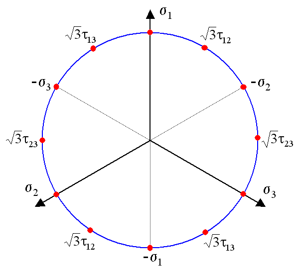
Graphical Representations
Here again is the sketch at the top of the page. It shows a bounding surface in a 3-D principal stress coordinate system where the von Mises stress is a constant value. (This is the so called High-Westerguard Space.) It is based on the fact that any stress state can be converted into its principal values and compared to this sketch. If the resulting principal stress point in the coordinate system is within the cylinder, then the material has not yielded. If it is on the surface, then the material has yielded. And if it is outside the cylinder, it means that you did an elastic analysis of a situation that cannot in fact be correct because yielding would have long since taken place.The remarkable result is that if you look down the \(\sigma_1 = \sigma_2 = \sigma_3\) axis, the cross-section of the cylinder is a perfect circle. Note that the hydrostatic stress in this situation does not show up at all.
Experimental Data
The figure here presents experimental data confirming that ductile metals yield much more consistently at prescribed von Mises stress levels regardless of the the loading state than at any other criteria.The graph represents a slice through the \(\sigma_1 - \sigma_2\) plane with \(\sigma_3 = 0\). Since the cylinder is cut at an angle, it appears to be an ellipse in this situation. It is in fact still a circle. We are just looking at it at an angle.
Recall that the shear stress criterion was first proposed by Tresca in 1864, and this act is considered to represent the birth of the field of metal plasticity research.
The one exception here is the cast iron metal. It yields, fractures in fact, at a constant maximum principal stress criterion. This signifies that the iron is brittle and behaves more like glass than a ductile metal.
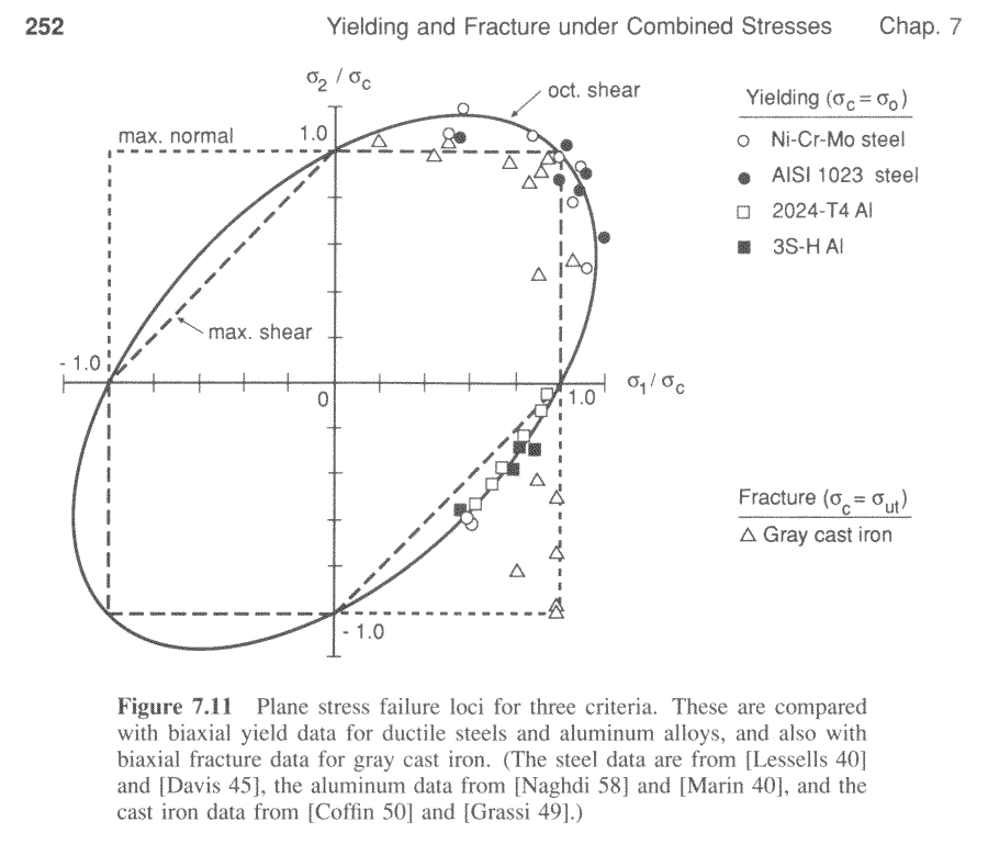
Reference: Dowling, N.E., Mechanical Behavior of Materials, Prentice Hall, 1993.
Note that the correlation here is not perfect. This is a consequence of the fact that the so-called von Mises Yield Criterion is NOT a law of nature. It is more of a convenient coincidence. It is a consequence of dislocation movement on millions and billions of planes of atoms sliding over each other at the atomic scale. Those planes of atoms are all randomly oriented, and the resulting response at the macroscale is.... the von Mises yield criterion.
Contrasting Stress and Strain
We've seen how the von Mises stress is "the stress" when worrying about metal yielding and plasticity. Recall that it is\[ \sigma_\text{VM} = \sqrt{ {3 \over 2} \boldsymbol{\sigma}' : \boldsymbol{\sigma}' } \]
The next question is, "Is there a strain analog to the von Mises stress?" The answer is yes. It is the effective strain, or sometimes the Mises effective strain. It is
\[ \epsilon_\text{eff} = \sqrt{ {2 \over 3} \boldsymbol{\epsilon}' : \boldsymbol{\epsilon}' } \]
Note that it is \(2/3\), not \(3/2\). This arises because the strain tensor for uniaxial tension of an incompressible material (which includes the plastic part of the total deformation of a metal) is
\[ \boldsymbol{\epsilon}_\text{True} = \left[ \matrix{ \epsilon & \;\;0 & \;\;0 \\ 0 & -{\epsilon \over 2} & \;\;0 \\ 0 & \;\;0 & -{\epsilon \over 2} } \right] \]
and \( \boldsymbol{\epsilon} : \boldsymbol{\epsilon} \) in this case gives \(3 \, \epsilon^2 / 2\). So it is necessary to multiply by \(2/3\) in order to make \( \boldsymbol{\epsilon}_\text{eff} \) equal to the uniaxial tension strain.
This makes it possible to more fairly compare the stress and strain states of two different deformation modes, say tension versus shear. In fact, in a perfectly isotropic metal, plots of effective stress versus effective strain will be indistinguishable in the plastic region regardless of the deformation mode. Although in reality, metals usually become increasingly anisotropic after yielding.
References
- Huber, M.T. (1904) Czasopismo Techniczne, Lemberg, Austria, Vol. 22, pp. 181.
- Von Mises, R. (1913) "Mechanik der Festen Korper im Plastisch Deformablen Zustand," Nachr. Ges. Wiss. Gottingen, pp. 582.
- Hencky, H.Z. (1924) "Zur Theorie Plasticher Deformationen und der Hierdurch im Material Hervorgerufenen Nachspannungen," Z. Angerw. Math. Mech., Vol. 4, pp. 323.
- Taylor, G.I., Quinney, H. (1931) "The Plastic Distortion of Metals," Phil. Trans. R. Soc., London, Vol. A230, pp. 323.
- Tresca, H. (1864) "Sur l'Ecoulement des Corps Solides Soumis a de Fortes Pressions," C. R. Acad. Sci., Paris, Vol. 59, pp. 754.
- Dowling, N.E. (1993) Mechanical Behavior of Materials, Prentice Hall.