Introduction
This page covers principal stresses and stress invariants. Everything here applies regardless of the type of stress tensor.Coordinate transformations of 2nd rank tensors were discussed on this coordinate transform page. The transform applies to any stress tensor, or strain tensor for that matter. It is written as
\[ \boldsymbol{\sigma}' = {\bf Q} \cdot \boldsymbol{\sigma} \cdot {\bf Q}^T \]
Everything below follows from two facts: First, the tensors are symmetric. Second, the above coordinate transformation is used.
2-D Principal Stresses
In 2-D, the transformation equations are\[ \begin{eqnarray} \sigma'\!_{xx} & = & \sigma_{xx} \cos^2 \theta + \sigma_{yy} \, \sin^2 \theta + 2 \, \tau_{xy} \, \sin \theta \cos \theta \\ \\ \sigma'\!_{yy} & = & \sigma_{xx} \sin^2 \theta + \sigma_{yy} \, \cos^2 \theta - 2 \, \tau_{xy} \, \sin \theta \cos \theta \\ \\ \tau'\!_{xy} & = & (\sigma_{yy} - \sigma_{xx}) \sin \theta \cos \theta + \tau_{xy} (\cos^2 \theta - \sin^2 \theta) \end{eqnarray} \]
The full shear stress values are used, unlike strain transformations, which use half values for shear strain, i.e., (\(\gamma / 2\)).
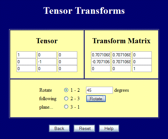
This page performs full 3-D tensor transforms, but can still be used for 2-D problems.. Enter values in the upper left 2x2 positions and rotate in the 1-2 plane to perform transforms in 2-D. The screenshot below shows a case of pure shear rotated 45° to obtain the principal stresses. Note also how the \({\bf Q}\) matrix transforms.
The figure below shows the stresses corresponding to the pure shear case in the tensor transform webpage example. The blue square aligned with the axes clearly undergoes shear. But the red square inscribed in the larger blue square only sees simple tension and compression. These are the principal values of the pure shear case in the global coordinate system.
In 2-D, the principal stress orientation, \(\theta_P\), can be computed by setting \(\tau'\!_{xy} = 0\) in the above shear equation and solving for \(\theta\) to get \(\theta_P\), the principal stress angle.
\[ 0 = (\sigma_{yy} - \sigma_{xx}) \sin \theta_P \cos \theta_P + \tau_{xy} (\cos^2 \theta_P - \sin^2 \theta_P) \]
\[ \tan (2 \theta_P) \; = \; {2 \tau_{xy} \over \sigma_{xx} - \sigma_{yy} } \]
The transformation matrix, \({\bf Q}\), is
\[ {\bf Q} = \left[ \matrix{ \;\;\; \cos \theta_P & \sin \theta_P \\ -\sin \theta_P & \cos \theta_P } \right] \]
Inserting this value for \(\theta_P\) back into the equations for the normal stresses gives the principal values. They are written as \(\sigma_{max}\) and \(\sigma_{min}\), or alternatively as \(\sigma_1\) and \(\sigma_2\).
\[ \sigma_{max}, \sigma_{min} = {\sigma_{xx} + \sigma_{yy} \over 2} \pm \sqrt{ \left( {\sigma_{xx} - \sigma_{yy} \over 2} \right)^2 + \tau_{xy}^2 } \]
They could also be obtained by using \(\boldsymbol{\sigma}' = {\bf Q} \cdot \boldsymbol{\sigma} \cdot {\bf Q}^T\) with \({\bf Q}\) based on \(\theta_P\).
Principal Stress Notation
Principal stresses can be written as \(\sigma_1\), \(\sigma_2\), and \(\sigma_3\). Only one subscript is usually used in this case to differentiate the principal stress values from the normal stress components: \(\sigma_{11}\), \(\sigma_{22}\), and \(\sigma_{33}\).2-D Principal Stress Example
Start with the stress tensor
\[ \boldsymbol{\sigma} = \left[ \matrix{ 50 & \;\;\; 30 \\ 30 & -20 } \right] \]
The principal orientation is
\[ \begin{eqnarray} \tan (2 \theta_P) & = & {2 * 30 \over 50 - (\text{-}20) } \\ \\ \\ \theta_P & = & 20.3° \end{eqnarray} \]
The principal stresses are
\[ \begin{eqnarray} \sigma_{max}, \sigma_{min} & = & {50 - 20 \over 2} \pm \sqrt{ \left( {50 + 20 \over 2} \right)^2 + (30)^2 } \\ \\ \\ \sigma_{max}, \sigma_{min} & = & 61.1, -31.1 \end{eqnarray} \]
The only limitation to using these equations for principal values is that it is not known which one applies to 20.3° and which applies to 110.3°. That's why an attractive alternative is
\[ \begin{eqnarray} \left[ \matrix{\sigma'\!_{11} & \sigma'\!_{12} \\ \sigma'\!_{12} & \sigma'\!_{22} } \right] & = & \left[ \matrix { \;\;\;\cos(20.3^\circ) & \sin(20.3^\circ) \\ -\sin(20.3^\circ) & \cos(20.3^\circ) } \right] \left[ \matrix{50 & \;\;\;30 \\ 30 & -20 } \right] \left[ \matrix { \cos(20.3^\circ) & -\sin(20.3^\circ) \\ \sin(20.3^\circ) & \;\;\;\cos(20.3^\circ) } \right] \\ \\ \\ & = & \left[ \matrix{61.1 & \;\;\;0.0 \\ 0.0 & -31.1 } \right] \end{eqnarray} \]
This confirms that the 61.1 principal stress value in the \(\sigma_{11}\) slot is indeed 20.3° from the X-axis. The \(\sigma_{22}\) value is 90° from the first.
3-D Principal Stresses
Coordinate transforms in 3-D are\[ \left[ \matrix{\sigma'_{11} & \sigma'_{12} & \sigma'_{13} \\ \sigma'_{12} & \sigma'_{22} & \sigma'_{23} \\ \sigma'_{13} & \sigma'_{23} & \sigma'_{33} } \right] = \left[ \matrix { q_{11} & q_{12} & q_{13} \\ q_{21} & q_{22} & q_{23} \\ q_{31} & q_{32} & q_{33} } \right] \left[ \matrix{\sigma_{11} & \sigma_{12} & \sigma_{13} \\ \sigma_{12} & \sigma_{22} & \sigma_{23} \\ \sigma_{13} & \sigma_{23} & \sigma_{33} } \right] \left[ \matrix { q_{11} & q_{21} & q_{31} \\ q_{12} & q_{22} & q_{32} \\ q_{13} & q_{23} & q_{33} } \right] \]
The second \({\bf Q}\) matrix is once again the transpose of the first.
This page performs tensor transforms.
And this page calculates principal values (eigenvalues) and principal directions (eigenvectors).
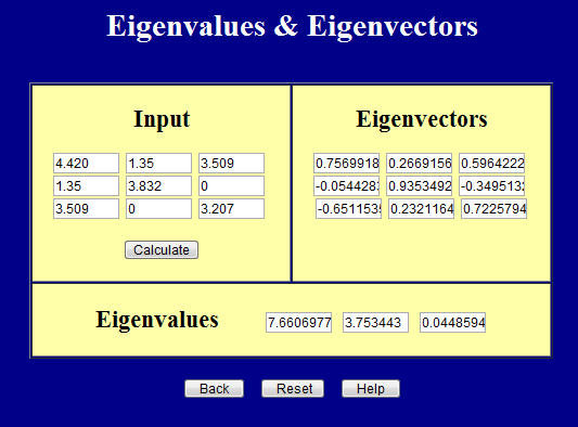
It's important to remember that the inputs to both pages must be symmetric. In fact, both pages enforce this.
The eigenvalues above can be written in matrix form as
\[ \boldsymbol{\sigma} = \left[ \matrix{ 24 & 0 & 0 \\ 0 & 125 & 0 \\ 0 & 0 & 433 } \right] \]
Maximum Shear Stress
The maximum shear stress at any point is easy to calculate from the principal stresses. It is simply\[ \tau_{max} = {\sigma_{max} - \sigma_{min} \over 2} \]
This applies in both 2-D and 3-D. The maximum shear always occurs in a coordinate system orientation that is rotated 45° from the principal coordinate system. For the principal stress tensor above
\[ \boldsymbol{\sigma} = \left[ \matrix{ 24 & 0 & 0 \\ 0 & 125 & 0 \\ 0 & 0 & 433 } \right] \]
The max and min principal stresses are in the \(\sigma_{33}\) and \(\sigma_{11}\) slots, respectively. So the max shear orientation is obtained by rotating the principal coordinate system by 45° in the (\(1-3\)) plane.
\[ \begin{eqnarray} \tau_{max} & = & {\sigma_{max} - \sigma_{min} \over 2} \\ \\ & = & (433 - 24) / 2 \\ \\ & = & 204 \end{eqnarray} \]
\[ \left| \matrix{\sigma_{11}-\lambda & \sigma_{12} & \sigma_{13} \\ \sigma_{12} & \sigma_{22}-\lambda & \sigma_{23} \\ \sigma_{13} & \sigma_{23} & \sigma_{33}-\lambda } \right| = 0 \]
This can be expanded out to give
\[ \begin{eqnarray} (\sigma_{11}-\lambda)\big[(\sigma_{22}-\lambda)(\sigma_{33}-\lambda)-\sigma^2_{23}\big] & - & \\ \sigma_{12}\big[\sigma_{12}(\sigma_{33}-\lambda)-\sigma_{23}\sigma_{13}\big] & + & \\ \sigma_{13}\big[\sigma_{12}\sigma_{23} - (\sigma_{22}-\lambda)\sigma_{13}\big] & = & 0 \end{eqnarray} \]
Invariants
...and expanded out even further to give\[ \begin{eqnarray} \lambda^3 - (\sigma_{11} + \sigma_{22} + \sigma_{33}) \lambda^2 + (\sigma_{11}\sigma_{22}+\sigma_{22}\sigma_{33}+\sigma_{33}\sigma_{11}-\sigma^2_{12}-\sigma^2_{13}-\sigma^2_{23}) \lambda - \\ (\sigma_{11}\sigma_{22}\sigma_{33}-\sigma_{11}\sigma^2_{23}-\sigma_{22}\sigma^2_{13}-\sigma_{33}\sigma^2_{12}+2\sigma_{12}\sigma_{13}\sigma_{23}) = 0 \end{eqnarray} \]
"Now consider this..."
No matter what coordinate transformation you apply to the stress tensor, its principal stress had better be the same three values. And the only way for this to happen in the above equation is for the equation itself to always be the same, no matter the transformation. This means that the combinations of stress components, which serve as coefficients of the \(\lambda\)'s, must be invariant under coordinate transformations. Their values must not change. And that's why they are called invariants.\[ \lambda^3 - I_1 \lambda^2 + I_2 \lambda - I_3 = 0 \]
where
\[ \begin{eqnarray} I_1 & = & \sigma_{11} + \sigma_{22} + \sigma_{33} \\ \\ I_2 & = & \sigma_{11}\sigma_{22}+\sigma_{22}\sigma_{33}+\sigma_{33}\sigma_{11}-\sigma^2_{12}-\sigma^2_{13}-\sigma^2_{23} \\ \\ I_3 & = & \sigma_{11}\sigma_{22}\sigma_{33}-\sigma_{11}\sigma^2_{23}-\sigma_{22}\sigma^2_{13}-\sigma_{33}\sigma^2_{12}+2\sigma_{12}\sigma_{13}\sigma_{23} \end{eqnarray} \]
Although probably not initially apparent, the invariants are actually familiar quantities.
\[ \begin{eqnarray} I_1 & = & \text{tr}(\boldsymbol{\sigma}) \\ \\ I_2 & = & \left| \matrix{\sigma_{11} & \sigma_{12} \\ \sigma_{12} & \sigma_{22}} \right| + \left| \matrix{\sigma_{11} & \sigma_{13} \\ \sigma_{13} & \sigma_{33}} \right| + \left| \matrix{\sigma_{22} & \sigma_{23} \\ \sigma_{23} & \sigma_{33}} \right| \\ \\ \\ I_3 & = & \text{det}(\boldsymbol{\sigma}) \end{eqnarray} \]
\[ \begin{eqnarray} I_1 & = & \sigma_{kk} \\ \\ I_2 & = & {1 \over 2} \left[ \left( \sigma_{kk} \right)^2 - \sigma_{ij} \sigma_{ij} \right] \\ \\ \\ I_3 & = & \epsilon_{ijk} \sigma_{i1} \sigma_{j2} \sigma_{k3} \end{eqnarray} \]
\(I_3\) is in tensor notation, but no one should actually calculate a determinant based on tensor notation rules because it is very inefficient.
Physical Interpretation of Invariants
The physical interpretation of the invariants depends on what tensor the invariants are computed from. For any stress or strain tensor, \(I_1\) is directly related to the hydrostatic component of that tensor. This is universal.\(I_2\) tends to be related more to the deviatoric aspects of stress and strain. For stress tensors, it is closely related to the von Mises stress.
Finally, \(I_3\) does not seem to have any physical significance as the determinant of a stress or strain tensor. But it does when applied to the deformation gradient. In that case, \(I_3 = V_F / V_o\), the ratio of deformed to initial volume, which is 1 for incompressible materials like rubber.
Invariant Example
This example will start with a random stress tensor and demonstrate that the invariants are indeed invariant under coordinate transformations. Start with the stress tensor\[ \boldsymbol{\sigma} = \left[ \matrix{ 50 & \;\;\; 30 & \;\;\;20 \\ 30 & -20 & -10 \\ 20 & -10 & \;\;\;10 } \right] \]
Its invariants are
\[ \begin{eqnarray} I_1 & = & 50 + (-20) + 10 \\ \\ & = & \;\;\;40 \\ \\ I_2 & = & (50)(-20) + (-20)(10) + (10)(50) - (30)^2 - (20)^2 - (-10)^2 \\ \\ & = & -2,100 \\ \\ I_3 & = & \text{det}(\boldsymbol{\sigma}) \\ \\ & = & -28,000 \end{eqnarray} \]
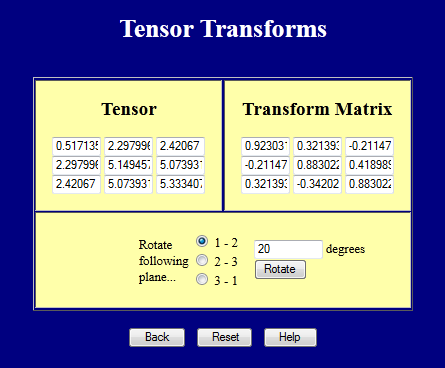
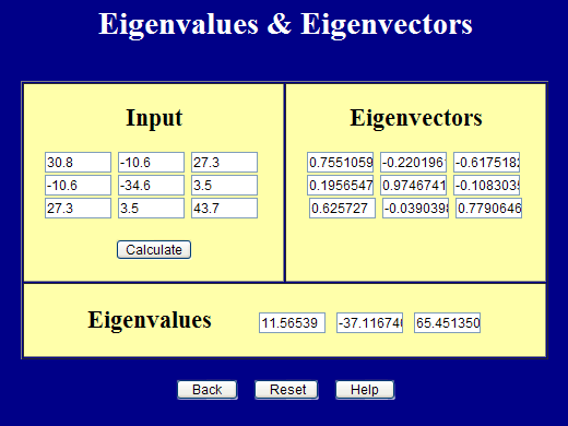
Now rotate the coordinate system by some random amount shown in the screenshot.
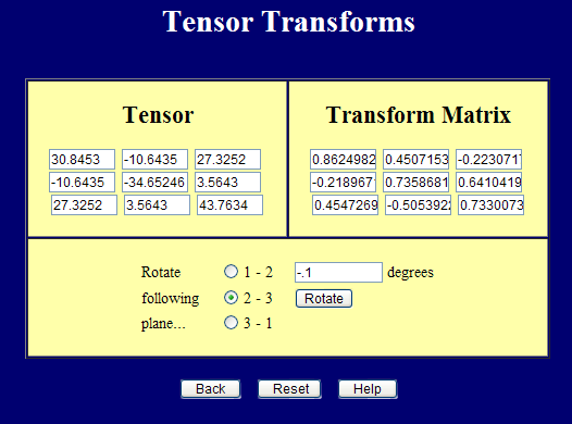
The transformed stress tensor is now
\[ \boldsymbol{\sigma} = \left[ \matrix{ \;\;\; 30.8 & -10.6 & 27.3 \\ -10.6 & -34.6 & 03.5 \\ \;\;\; 27.3 & \;\;\;3.5 & 43.7 } \right] \]
And the "new" invariants are
\[ \begin{eqnarray} I_1 & = & 30.8 + (-34.6) + 43.7 \\ & = & \;\;\;40 \\ \\ I_2 & = & (30.8)(-34.6) + (-34.6)(43.7) + (43.7)(30.8) - (-10.6)^2 - (27.3)^2 - (3.5)^2 \\ & = & -2,100 \\ \\ I_3 & = & \text{det}(\boldsymbol{\sigma}) \\ & = & -28,000 \end{eqnarray} \]
So they are indeed invariant.
Just for grins... Let's compute the principal stresses and then recompute the invariants to demonstrate again that they are invariant.
The principal stresses are
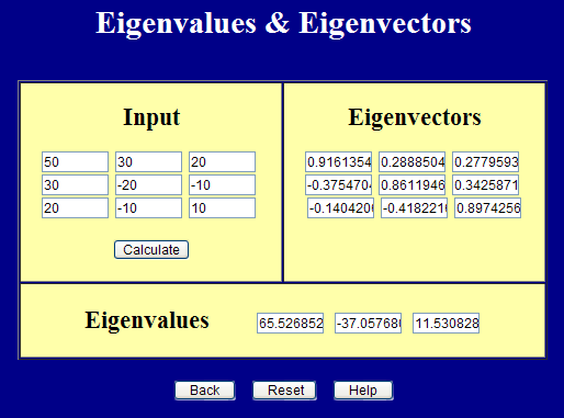
\[ \boldsymbol{\sigma}' = \left[ \matrix{ 65.5 & 0 & 0 \\ 0 & -37.1 & 0 \\ 0 & 0 & 11.5 } \right] \]
Curiously, the two different starting points lead to the principal values being listed in different orders. This is typical and has no special meaning. The final, physical answer is the same. The \({\bf Q}\) will accommodate the different listing orders.
Finally, calculating the invariants one last time using the principal values gives
\[ \begin{eqnarray} I_1 & = & 65.5 + (-37.1) + 11.5 \\ \\ & = & \;\;\;40 \\ \\ I_2 & = & (65.5)(-37.1) + (-37.1)(11.5) + (11.5)(65.5) \\ \\ & = & -2,100 \\ \\ I_3 & = & \text{det}(\boldsymbol{\sigma}') \quad = \quad (65.5)(-37.1)(11.5) \\ \\ & = & -28,000 \end{eqnarray} \]
And so it works again. Note how the invariant calculations are rather simple when all the off-diagonal terms are zero. The determinant is especially easy.
2-D Invariants
In the 2-D world, there are only two invariants.\[ \begin{eqnarray} I_1 & = & \text{tr}(\boldsymbol{\sigma}) & = & \sigma_{11} + \sigma_{22} \\ \\ I_2 & = & \text{det}(\boldsymbol{\sigma}) & = & \sigma_{11} * \sigma_{22} - \sigma^2_{12} \\ \end{eqnarray} \]
In 2-D, things are just simple enough to directly prove the invariance of invariants. We'll prove it for \(I_1\) here. Recall the transformation equations are
\[ \begin{eqnarray} \sigma'\!_{xx} & = & \sigma_{xx} \cos^2 \theta + \sigma_{yy} \, \sin^2 \theta + 2 \tau_{xy} \sin \theta \cos \theta \\ \\ \sigma'\!_{yy} & = & \sigma_{xx} \sin^2 \theta + \sigma_{yy} \, \cos^2 \theta - 2 \tau_{xy} \sin \theta \cos \theta \\ \\ \tau'\!_{xy} & = & (\sigma_{yy} - \sigma_{xx}) \sin \theta \cos \theta + \tau_{xy} (\cos^2 \theta - \sin^2 \theta) \end{eqnarray} \]
So \(\sigma'\!_{xx} + \sigma'\!_{yy}\) is
\[ \begin{eqnarray} \sigma'\!_{xx} + \sigma'\!_{yy} & = & \sigma_{xx} \cos^2 \theta + \sigma_{yy} \, \sin^2 \theta + 2 \tau_{xy} \sin \theta \cos \theta + \\ \\ & & \sigma_{xx} \sin^2 \theta + \sigma_{yy} \, \cos^2 \theta - 2 \tau_{xy} \sin \theta \cos \theta \\ \end{eqnarray} \]
and the shear terms cancel, while the normal stress terms combine to give
\[ \begin{eqnarray} \sigma'\!_{xx} + \sigma'\!_{yy} & = & \sigma_{xx} ( \cos^2 \theta + \sin^2 \theta ) + \sigma_{yy} ( \sin^2 \theta + \cos^2 \theta ) \\ \\ & = & \sigma_{xx} + \sigma_{yy} \end{eqnarray} \]
So it works again.
Calculating Principal Values Manually in 3-D
Here's how to compute the roots of a cubic equation... applied to principal values. Start with\[ \lambda^3 - I_1 \lambda^2 + I_2 \lambda - I_3 = 0 \]
Recall that the resulting \(\lambda's\) will be the principal values of the stress or strain tensor... and the invariants will need to be calculated up front.
The first step is to calculate two intermediate quantities, \(Q\) and \(R\).
\[ Q = { 3 I_2 - I^2_1 \over 9 } \qquad R = {2 I^3_1 - 9 I_1 I_2 + 27 I_3 \over 54} \]
Then calculate another intermediate quantity, \(\theta\).
\[ \theta = \text{cos}^{-1} \left( R \over \sqrt{-Q^3} \right) \]
\[ \begin{eqnarray} \epsilon_1 & = & 2 \, \sqrt{-Q} \, \cos \left( {\theta \over 3} \right) & + & {1\over 3} I_1 \\ \\ \\ \epsilon_2 & = & 2 \, \sqrt{-Q} \, \cos \left( {\theta + 2 \pi \over 3} \right) & + & {1\over 3} I_1 \\ \\ \\ \epsilon_3 & = & 2 \, \sqrt{-Q} \, \cos \left( {\theta + 4 \pi \over 3} \right) & + & {1\over 3} I_1 \end{eqnarray} \]
Note that minus signs are easily confused here because they are present in the original cubic invariant equation being solved.
Ref: http://mathworld.wolfram.com/CubicFormula.html
Summary
This principle of invariant quantities under coordinate transformations is in fact universal across all matrices that are symmetric and being transformed according to\[ {\bf A}' = {\bf Q} \cdot {\bf A} \cdot {\bf Q}^T \]
where \({\bf A}\) is "any symmetric matrix."
And recall that the product of any matrix with its transpose is always a symmetric result, so this result would qualify. This is especially relevant to \({\bf F}^T \! \cdot {\bf F}\), whose invariants are used in the Mooney-Rivlin Law of rubber behavior. Mooney-Rivlin's Law and coefficients will be discussed on this page. As an added teaser, we will see that the 3rd invariant of \({\bf F}^T \! \cdot {\bf F}\) for rubber always equals 1 because rubber is incompressible. So not only is it a constant, independent of coordinate transformations, but it is even a constant value, always equal to 1, independent of coordinate transformations and the state of deformation.