Introduction
This page supplements the previous coordinate transformation page by focusing on the many ways to generate and interpret the transformation matrix, \({\bf Q}\). Remember, one more time, that the transform matrix rotates the coordinate system, not the object.Quick Review
The transformation matrix, \({\bf Q}\), is used in coordinate transformations of vectors and tensors as follows.| Vectors | \({\bf v'}\) | \( = \) | \({\bf Q} \cdot {\bf v}\) | |
| 2nd Rank Tensors | \(\boldsymbol{\sigma'}\) | \( = \) | \({\bf Q} \cdot \boldsymbol{\sigma} \cdot {\bf Q}^T\) | |
| 4th Rank Tensors | \({\bf C'}\) | \( = \) | \({\bf Q} \cdot {\bf Q} \cdot {\bf C} \cdot {\bf Q}^T \cdot {\bf Q}^T\) |
and in tensor notation...
| Vectors | \(v'_i\) | \( = \) | \(\lambda_{ij} v_j\) | |
| 2nd Rank Tensors | \(\sigma'_{mn}\) | \( = \) | \(\lambda_{mi} \lambda_{nj} \sigma_{ij}\) | |
| 4th Rank Tensors | \(C'_{mnop}\) | \( = \) | \(\lambda_{mi} \lambda_{nj} \lambda_{ok} \lambda_{pl} C_{ijkl} \) |
In two dimensions, \({\bf Q}\) is
\[ {\bf Q} = \left[ \matrix {\;\;\;\cos \theta & \sin \theta \\ -\sin \theta & \cos \theta} \right] \]
where \(\theta\) is the angle between the old and new axes. This is simply a special case of the general 3-D case discussed below.
Transformation Matrix Properties
Transformation matrices have several special properties that, while easily seen in this discussion of 2-D vectors, are equally applicable to 3-D applications as well. This list is useful for checking the accuracy of a transformation matrix if questions arise. While a matrix still could be wrong even if it passes all these checks, it is definitely wrong if it fails even one!
|
\[ {\bf Q} = \left[ \matrix {\;\;\;\cos \theta & \sin \theta \\ -\sin \theta & \cos \theta} \right] \] |
Multiplication of Transformation Matrices
Recall from above that the dot product of any two different rows or columns of a transformation matrix is zero, while the dot product of any row or column with itself is one. This can be written in matrix and tensor notation as\[ {\bf Q} \cdot {\bf Q}^T = {\bf I} \qquad \qquad \text{and} \qquad \qquad \lambda_{ik} \lambda_{jk} = \delta_{ij} \]
This shows that the transpose of a transformation matrix is also its inverse.
\[ {\bf Q} = \left[ \matrix { \cos(x',x) & \cos(x',y) & \cos(x',z) \\ \cos(y',x) & \cos(y',y) & \cos(y',z) \\ \cos(z',x) & \cos(z',y) & \cos(z',z) } \right] \]
where \((x',x)\) represents the angle between the \(x'\) and \(x\) axes, \((x',y)\) is the angle between the \(x'\) and \(y\) axes, etc.
3-D Reduction to 2-D
So a rotation about the \(z\)-axis means that \(\cos(z',z) = 1\) because the angle between \(z'\) and \(z\) remains 0°. Meanwhile, \(\cos(x',z) = \cos(y',z) = \cos(z',x) = \cos(z',y) = 0\) because the angles between these axes remains 90°.The angle between \(x'\) and \(y\) is \((90^\circ - \theta)\), and \(\cos(x',y) = \cos(90^\circ - \theta) = \sin \theta\).
Likewise, the angle between \(y'\) and \(x\) is \((90^\circ + \theta)\), and \(\cos(y',x) = \cos(90^\circ + \theta) = -\sin \theta\).
All of this leads to
\[ {\bf Q} = \left[ \matrix { \;\;\; \cos \theta & \sin \theta & 0 \\ -\sin \theta & \cos \theta & 0 \\ 0 & 0 & 1 } \right] \]
which reveals the 2-D transformation matrix within the 3-D matrix.
An alternative way of interpreting and generating the transformation matrix is as follows.
\[ {\bf Q} = \left[ \matrix { \left( \matrix{\text{x-comp} \\ \text{of } {\bf i'}} \right) & \left( \matrix{\text{y-comp} \\ \text{of } {\bf i'}} \right) & \left( \matrix{\text{z-comp} \\ \text{of } {\bf i'}} \right) \\ \left( \matrix{\text{x-comp} \\ \text{of } {\bf j'}} \right) & \left( \matrix{\text{y-comp} \\ \text{of } {\bf j'}} \right) & \left( \matrix{\text{z-comp} \\ \text{of } {\bf j'}} \right) \\ \left( \matrix{\text{x-comp} \\ \text{of } {\bf k'}} \right) & \left( \matrix{\text{y-comp} \\ \text{of } {\bf k'}} \right) & \left( \matrix{\text{z-comp} \\ \text{of } {\bf k'}} \right) } \right] \]
where "x-comp of \({\bf i'}\)" means the x-component of the \({\bf i'}\) unit vector. Pay close attention here to which terms have primes on them and which don't. Don't confuse this with "the x'-component" because "the x'-comp of \({\bf i'}\)" is simply 1. Yet another way to say this is, "the first component of the \({\bf i'}\) unit vector in the non-primed reference \(x, y, z\) coordinate system."
Transformation Webpage
This webpage performs coordinate transforms on 3-D tensors. It also reports the transformation matrix. Try it out. Note that rotations on the webpage are always about global axes, e.g., a rotation in the 1-2 plane will be about the 3-axis.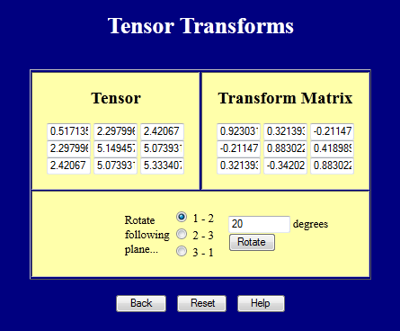
Successive Rotations - Roe Convention
The 3-D transformation matrix can be viewed as a series of three successive rotations about coordinate axes. There must be dozens of variations of this since any combination of axes can be chosen in any order to rotate about. One popular choice is the so-called Roe convention.As shown in the figure, it consists of (i) a rotation through angle \(\psi\) about the z-axis, then (ii) a rotation of angle \(\theta\) about the new y-axis (which has already rotated itself due to the first rotation about z), and finally, (iii) a second rotation of \(\phi\) about the now-tilted z-axis.
The Roe convention is very popular despite one key challenge it contains. That is... if \(\theta = 0\), then \(\psi\) and \(\phi\) become indistinguishable and only the sum of the two is what matters.
\[ \begin{eqnarray} {\bf Q} & = & \left[ \matrix { \;\;\; \cos \phi & \sin \phi & 0 \\ -\sin \phi & \cos \phi & 0 \\ 0 & 0 & 1 } \right] \left[ \matrix { \cos \theta & 0 & -\sin \theta \\ 0 & 1 & 0 \\ \sin \theta & 0 & \;\;\; \cos \theta } \right] \left[ \matrix { \;\;\; \cos \psi & \sin \psi & 0 \\ -\sin \psi & \cos \psi & 0 \\ 0 & 0 & 1 } \right] \\ \\ \\ & = & \left[ \matrix { \;\;\; \cos \psi \cos \theta \cos \phi - \sin \psi \sin \phi & \;\;\; \sin \psi \cos \theta \cos \phi + \cos \psi \sin \phi & -\sin \theta \cos \phi \\ -\cos \psi \cos \theta \sin \phi - \sin \psi \cos \phi & -\sin \psi \cos \theta \sin \phi + \cos \psi \cos \phi & \;\;\; \sin \theta \sin \phi \\ \cos \psi \sin \theta & \sin \psi \sin \theta & \cos \theta } \right] \end{eqnarray} \]
Even though the rotation angles are applied in \(\psi, \theta, \phi\) order, the matrices are indeed written in the opposite order: \(\phi, \theta, \psi\).
Roe Angles Example
In the figure above, \(\psi = 60^\circ, \theta = 30^\circ,\) and \(\phi = 45^\circ\). These Roe angles give a coordinate transformation matrix equal to\[ \begin{eqnarray} {\bf Q} & = & \left[ \matrix { \;\;\; \cos 60^\circ \cos 30^\circ \cos 45^\circ - \sin 60^\circ \sin 45^\circ & \;\;\; \sin 60^\circ \cos 30^\circ \cos 45^\circ + \cos 60^\circ \sin 45^\circ & -\sin 30^\circ \cos 45^\circ \\ -\cos 60^\circ \cos 30^\circ \sin 45^\circ - \sin 60^\circ \cos 45^\circ & -\sin 60^\circ \cos 30^\circ \sin 45^\circ + \cos 60^\circ \cos 45^\circ & \;\;\; \sin 30^\circ \sin 45^\circ \\ \cos 60^\circ \sin 30^\circ & \sin 60^\circ \sin 30^\circ & \cos 30^\circ } \right] \\ \\ \\ & = & \left[ \matrix { -0.3062 & \;\;\; 0.8839 & -0.3536 \\ -0.9186 & -0.1768 & \;\;\; 0.3536 \\ \;\;\; 0.2500 & \;\;\; 0.4330 & \;\;\; 0.8660 } \right] \end{eqnarray} \]
Going In Reverse - Determining Roe Angles from a Matrix
\[ {\bf Q} = \left[ \matrix { q_{11} & q_{12} & q_{13} \\ q_{21} & q_{22} & q_{23} \\ q_{31} & q_{32} & q_{33} } \right] \]
The first and easiest step is to look at the \(q_{33}\) component. It is simply the cosine of \(\theta\), so \(\theta = \text{Cos}^{-1}(q_{33})\).
The second step is to determine \(\psi\) as follows
\[ {q_{32} \over q_{31}} = { \sin \psi \sin \theta \over \cos \psi \sin \theta } = { \sin \psi \over \cos \psi } = \tan \psi \] So
\[ \psi = \text{Tan}^{-1} \left( {q_{32} \over q_{31}} \right) \] \(\phi\) is determined in a very similar manner.
\[ {q_{23} \over -q_{13}} = { \sin \theta \sin \phi \over \sin \theta \cos \phi } = { \sin \phi \over \cos \phi } = \tan \phi \]
So
\[ \phi = \text{Tan}^{-1} \left({q_{23} \over -q_{13}} \right) \] In summary
\[ \psi = \text{Tan}^{-1} \left( {q_{32} \over q_{31}} \right) \qquad \qquad \theta = \text{Cos}^{-1} \left( q_{33} \right) \qquad \qquad \phi = \text{Tan}^{-1} \left({q_{23} \over -q_{13}} \right) \]
UNLESS!!!....... \(\theta\) proves to be very small! In this case, \(\sin \theta\) will be very small and therefore, so will \(q_{13}, q_{23}, q_{31}\), and \(q_{32}\) because all these terms contain \(\sin \theta\). This can lead to major round-off errors in any such calculations.
Fortunately, the solution for this (\(\theta \rightarrow 0\)) is to recall that \(\psi\) and \(\phi\) become indistinguishable from each other. This permits \(\phi\) to be set to zero, and \(\psi\) to be computed according to \(\psi = \text{Sin}^{-1}(q_{12})\).
Example: Roe Angles from Matrix
Let's start with the matrix in the previous example and work backwards.\[ {\bf Q} = \left[ \matrix { -0.3062 & \;\;\; 0.8839 & -0.3536 \\ -0.9186 & -0.1768 & \;\;\; 0.3536 \\ \;\;\; 0.2500 & \;\;\; 0.4330 & \;\;\; 0.8660 } \right] \]
Start with the \(q_{33}\) term to determine \(\theta\).
\[ \theta = \text{Cos}^{-1}(q_{33}) = \text{Cos}^{-1}(0.8660) = 30^\circ \]
Since \(\theta\) is not near zero, \(\psi\) and \(\phi\) can be computed as follows.
\[ \psi = \text{Tan}^{-1}\left({q_{32} \over q_{31}}\right) = \text{Tan}^{-1}\left({0.4330 \over 0.2500}\right) = 60^\circ \]
\[ \phi = \text{Tan}^{-1}\left({q_{23} \over -q_{13}}\right) = \text{Tan}^{-1}\left({0.3536 \over 0.3536}\right) = 45^\circ \]
So as expected, the original values are recovered: \( \psi = 60^\circ, \; \theta = 30^\circ,\) and \(\phi = 45^\circ\).
Rotation About An Axis
Yet another way of specifying the orientation of a transformed coordinate system is through a rotation axis vector, \({\bf p}\), and a rotation angle, \(\alpha\), about the \({\bf p}\) axis.
In this case, the transformation matrix is written as
\[ {\bf Q} = \cos \alpha \; {\bf I} + (1 - \cos \alpha) {\bf p} \otimes {\bf p} + \sin \alpha \; {\bf P} \]
with
\[ {\bf P} = \left[ \matrix { \;\;\; 0 & \;\;\; p_3 & -p_2 \\ -p_3 & \;\; 0 & \;\;\; p_1 \\ \;\;\; p_2 & -p_1 & \;\;\; 0 } \right] \]
Writing the matrix out gives
\[ {\bf Q} = \left[ \matrix { \cos \alpha + (1-\cos \alpha) p^2_1 & (1 - \cos \alpha) p_1 p_2 + \sin \alpha \; p_3 & (1 - \cos \alpha) p_1 p_3 - \sin \alpha \; p_2 \\ (1 - \cos \alpha) p_2 p_1 - \sin \alpha \; p_3 & \cos \alpha + (1-\cos \alpha) p^2_2 & (1 - \cos \alpha) p_2 p_3 + \sin \alpha \; p_1 \\ (1 - \cos \alpha) p_3 p_1 + \sin \alpha \; p_2 & (1 - \cos \alpha) p_3 p_2 - \sin \alpha \; p_1 & \cos \alpha + (1-\cos \alpha) p^2_3 } \right] \]
As usual, this can be written quite concisely in tensor notation
\[ Q_{ij} = \cos \alpha \; \delta_{ij} + (1 - \cos \alpha) p_i p_j + \sin \alpha \; \epsilon_{ijk} \; p_k \]
It is very important to recognize that \({\bf p}\) is a unit vector. Using any other length will lead to incorrect results.
Also, it's actually more common to use \(\theta\) or \(\phi\) as the rotation angle instead of \(\alpha\). But \(\alpha\) is being used here to minimize confusion with \(\psi, \theta,\) and \(\phi\) used as the Roe convention angles.
It is easy to visualize the coordinate rotations in this method. For example, the 2-D case can be reproduced by noting that the rotation is about the z-axis, so the vector is \({\bf p} = (0, 0, 1)\). This leads to
\[ {\bf Q} = \left[ \matrix { \;\;\; \cos \alpha & \sin \alpha & 0 \\ -\sin \alpha & \cos \alpha & 0 \\ 0 & 0 & 1 } \right] \]
\[ \alpha = \text{Cos}^{-1} \left\{ {1 \over 2} \Big[ \text{tr}({\bf Q}) - 1 \Big] \right\} \]
Once \(\alpha\) is determined, the components of \({\bf p}\) are computed by
\[ p_1 = { q_{23} - q_{32} \over 2 \sin \alpha } \qquad \qquad p_2 = { q_{31} - q_{13} \over 2 \sin \alpha } \qquad \qquad p_3 = { q_{12} - q_{21} \over 2 \sin \alpha } \]
The three equations can be conveniently summarized in tensor notation as
\[ p_i = { \epsilon_{ijk} \, q_{jk} \over 2 \sin \alpha} \]
Note that \({\bf p}\) becomes undefined when \(\alpha = 0\). This means, "the axis you rotate about doesn't matter if you don't rotate in the first place."
Backing Out P and α
Determine the single rotation, \({\bf p}\) and \(\alpha\), that is equivalent to that produced by the Roe angles used earlier: \(\psi = 60^\circ, \theta = 30^\circ,\) and \(\phi = 45^\circ\).Recall that the Roe angles \(\psi = 60^\circ, \theta = 30^\circ,\) and \(\phi = 45^\circ\) lead to
\[ {\bf Q} = \left[ \matrix { -0.3062 & \;\;\; 0.8839 & -0.3536 \\ -0.9186 & -0.1768 & \;\;\; 0.3536 \\ \;\;\; 0.2500 & \;\;\; 0.4330 & \;\;\; 0.8660 } \right] \]
Solving for \(\alpha\) gives
\[ \alpha = \text{Cos}^{-1} \left\{ {1 \over 2} \Big[ -0.3062 - 0.1768 +0.8660 - 1 \Big] \right\} = 108^\circ \]
\[ \begin{eqnarray} p_1 &=& \;\;\; { 0.3536 - 0.4330 \over 2 \; \sin 108^\circ} &=& -0.0417\\ \\ p_2 &=& { 0.2500 - (-0.3536) \over 2 \; \sin 108^\circ} &=& \;\;\; 0.3173\\ \\ p_3 &=& { 0.8839 - (-0.9186) \over 2 \; \sin 108^\circ} &=& \;\;\; 0.9475 \end{eqnarray} \]
So the Roe angles \(\psi = 60^\circ, \theta = 30^\circ,\) and \(\phi = 45^\circ\) are equivalent to a single rotation of \(108^\circ\) about the axis given by \({\bf p} = (-0.0417\), \(0.3173\), \(0.9475)\). Both sets lead to the new \(x', y', z'\) axes pointing in the same directions.
Inverses and Transposes
All coordinate transformation matrices possess a rather remarkable property - their transpose is their inverse. So it becomes trivial to compute the inverse of such a matrix.\[ {\bf Q}^T = {\bf Q}^{-1} \qquad \text{so} \qquad {\bf Q}^T \cdot {\bf Q} = {\bf I} \]
Transpose Product Example
The above \({\bf Q}\) matrix is\[ {\bf Q} = \left[ \matrix { -0.3062 & \;\;\; 0.8839 & -0.3536 \\ -0.9186 & -0.1768 & \;\;\; 0.3536 \\ \;\;\; 0.2500 & \;\;\; 0.4330 & \;\;\; 0.8660 } \right] \]
Multiply it by its transpose to demonstrate that the result is the identity matrix and therefore, its transpose must also be its inverse.
\[ {\bf Q}^T \cdot {\bf Q} = \left[ \matrix { -0.3062 & -0.9186 & 0.2500 \\ \;\;\; 0.8839 & -0.1768 & 0.4330 \\ -0.3536 & \;\;\; 0.3536 & 0.8660 } \right] \; \left[ \matrix { -0.3062 & \;\;\; 0.8839 & -0.3536 \\ -0.9186 & -0.1768 & \;\;\; 0.3536 \\ \;\;\; 0.2500 & \;\;\; 0.4330 & \;\;\; 0.8660 } \right] = \left[ \matrix { 1 & 0 & 0 \\ 0 & 1 & 0 \\ 0 & 0 & 1 } \right] \]