Introduction
Coordinate transformations are nonintuitive enough in 2-D, and positively painful in 3-D. This page tackles them in the following order: (i) vectors in 2-D, (ii) tensors in 2-D, (iii) vectors in 3-D, (iv) tensors in 3-D, and finally (v) 4th rank tensor transforms.A major aspect of coordinate transforms is the evaluation of the transformation matrix, especially in 3-D. This is touched on here, and discussed at length on the next page.
It is very important to recognize that all coordinate transforms on this page are rotations of the coordinate system while the object itself stays fixed. The "object" can be a vector such as force or velocity, or a tensor such as stress or strain in a component. Object rotations are discussed in later sections.
2-D Coordinate Transforms of Vectors
The academic potato provides an excellent example of how coordinate transformations apply to vectors, while at the same time stressing that it is the coordinate system that is rotating and not the vector... or potato.The potato on the left has a vector on it. But without a coordinate system, there is no way to describe the vector. So a coordinate system has been added to the potato as shown on the right, allowing the vector to now be described as \({\bf v} = 2{\bf i} + 9{\bf j}\).
So now we introduce a rotated coordinate system shown in blue below, using \(x'\) and \(y'\). The new system is rotated counter-clockwise by an angle, \(\theta\), from the initial coordinate system. Note that the vector itself does not change at all. It is still the very same vector as before. But it is described by different numerical values in the new coordinate system. In this case, the vector is more closely parallel to the new \(x'\) axis than the \(y'\) axis, so the \({\bf i'}\) component will be greater than the \({\bf j'}\) component. The transformation is given below the figure.
\[ v'_x = \;\;\; v_x \cos \theta + v_y \sin \theta \] \[ v'_y = -v_x \sin \theta + v_y \cos \theta \]
This can be seen by noting that
- the part of \(v_x\) that lies along the \(x'\) axis is \(v_x \cos \theta\)
- the part of \(v_y\) that lies along the \(x'\) axis is \(v_y \sin \theta\)
- the part of \(v_x\) that lies along the \(y'\) axis is \(-v_x \sin \theta\)
- the part of \(v_y\) that lies along the \(y'\) axis is \(v_y \cos \theta\)
Returning to the Potato...
So, if \(\theta = 50^\circ\), then\[ v'_x = \;\;\; 2 \cos 50^\circ + 9 \sin 50^\circ = 8.18 \] \[ v'_y = -2 \sin 50^\circ + 9 \cos 50^\circ = 4.25 \]
The \(v'_x\) component is indeed greater than the \(v'_y\) component as expected.
Transformation Matrix
\[ \left\{ \matrix {v'_x \\ v'_y} \right\} = \left[ \matrix {\;\;\;\cos \theta & \sin \theta \\ -\sin \theta & \cos \theta} \right] \left\{ \matrix {v_x \\ v_y} \right\} \]
The \(\cos \theta\) terms are on the matrix diagonal while the \(\sin \theta\) terms are off-diagonal. The only potential gotcha is remembering which \(\sin \theta\) term has the minus sign on it. It is always the lower-left term.
The above equation is written in matrix notation as
\[ {\bf v'} = {\bf Q} \cdot {\bf v} \]
where \({\bf Q}\) is the usual letter chosen for the transformation matrix.
Transformation vs Rotation Matrices
If this topic weren't already difficult enough, many books and websites add to the confusion by not clarifying what is fixed and what is rotating. In this page and the next, it is the coordinate system that is rotating while the object remains fixed. So the term transformation matrix is used here to emphasize this.However, we will later address situations in which the object rotates while the coordinate system remains fixed. In this scenario, the term rotation matrix will be used to emphasize that the object is rotating.
Much confusion arises from the amazing fact that each matrix (transform and rotation) is just the transpose of the other! So they look extremely similar. In 2-D problems, the only practical difference is whether the minus sign in front of \(\sin \theta\) is on the \(q_{12}\) term, or the \(q_{21}\) term.
Transformation Matrix Properties
Transformation matrices have several special properties that, while easily seen in this discussion of 2-D vectors, are equally applicable to 3-D applications as well. This list is useful for checking the accuracy of a transformation matrix if questions arise. While a matrix still could be wrong even if it passes all these checks, it is definitely wrong if it fails even one!
|
\[ {\bf Q} = \left[ \matrix {\;\;\;\cos \theta & \sin \theta \\ -\sin \theta & \cos \theta} \right] \] |
\[ {\bf Q} = \left[ \matrix { \cos(x',x) & \cos(x',y) \\ \cos(y',x) & \cos(y',y) } \right] \]
where \((x',x)\) represents the angle between the \(x'\) and \(x\) axes, \((x',y)\) is the angle between the \(x'\) and \(y\) axes, etc.
The angle between \(x'\) and \(y\) is \((90^\circ - \theta)\), and \(\cos(x',y) = \cos(90^\circ - \theta) = \sin \theta\).
Likewise, the angle between \(y'\) and \(x\) is \((90^\circ + \theta)\), and \(\cos(y',x) = \cos(90^\circ + \theta) = -\sin \theta\).
Transformation Matrix Formulation
Another way of building up the transformation matrix (and my favorite) is as follows\[ {\bf Q} = \left[ \matrix { \left( \matrix{\text{x-comp} \\ \text{of } {\bf i'}} \right) & \left( \matrix{\text{y-comp} \\ \text{of } {\bf i'}} \right) \\ \left( \matrix{\text{x-comp} \\ \text{of } {\bf j'}} \right) & \left( \matrix{\text{y-comp} \\ \text{of } {\bf j'}} \right) } \right] \]
"x-comp of \({\bf i'}\)" means the x-component of the \({\bf i'}\) unit vector. Pay close attention to which terms have primes on them and which don't. Don't confuse this with "the x'-component" because "the x'-comp of \({\bf i'}\)" is simply 1. Yet another way to say this is, "the first component of the \({\bf i'}\) unit vector in the non-primed reference \(x-y\) coordinate system."
In summary,
- the x-comp of \({\bf i'}\) is \(\cos \theta\)
- the y-comp of \({\bf i'}\) is \(\sin \theta\)
- the x-comp of \({\bf j'}\) is \(-\sin \theta\)
- the y-comp of \({\bf j'}\) is \(\cos \theta\)
Tensor Notation
\[ v'_i = \lambda_{ij} v_j \]
where \(\lambda_{ij}\) is the transformation matrix \({\bf Q}\). (I don't know why \({\bf Q}\) is used in matrix notation, but \(\lambda_{ij}\), not \(q_{ij}\), is used in tensor notation.) \(\lambda_{ij}\) is defined as
\[ \lambda_{ij} = \cos(x'_i,x_j) \]
For example, if \(i = 1\) and \(j = 2\), then
\[ \lambda_{12} = \cos(x'_1,x_2) = \cos(x',y) \]
\(\lambda_{ij}\) is the direction cosine of the angle between the \(x'_i\) axis and the \(x_j\) axis. Again, this is equally applicable to 3-D transformations as well.
Multiplication of Transformation Matrices
Recall from above that the dot product of any two different rows or columns of a transformation matrix is zero, while the dot product of any row or column with itself is one. This can be written in matrix and tensor notation as\[ {\bf Q} \cdot {\bf Q}^T = {\bf I} \qquad \qquad \text{and} \qquad \qquad \lambda_{ik} \lambda_{jk} = \delta_{ij} \]
This shows that the transpose of a transformation matrix is also it's inverse.
2-D Coordinate Transforms of Tensors
Coordinate transformations of 2nd rank tensors involve the very same \({\bf Q}\) matrix as vector transforms. A transformation of the stress tensor, \(\boldsymbol{\sigma}\), from the reference \(x-y\) coordinate system to \(\boldsymbol{\sigma'}\) in a new \(x'-y'\) system is done as follows.
\[ \boldsymbol{\sigma'} = {\bf Q} \cdot \boldsymbol{\sigma} \cdot {\bf Q}^T \]
Writing the matrices out explicitly gives
\[ \left[ \matrix{\sigma'_{xx} & \sigma'_{xy} \\ \sigma'_{xy} & \sigma'_{yy} } \right] = \left[ \matrix{\;\;\; \cos \theta & \sin \theta \\ -\sin \theta & \cos \theta } \right] \left[ \matrix{\sigma_{xx} & \sigma_{xy} \\ \sigma_{xy} & \sigma_{yy} } \right] \left[ \matrix{\cos \theta & -\sin \theta \\ \sin \theta & \;\;\; \cos \theta } \right] \]
(Note that the stress tensor is always symmetric, even following transformations.)
Multiplying the matrices out gives
\[ \begin{eqnarray} \sigma'_{xx} & = & \sigma_{xx} \cos^2 \theta + \sigma_{yy} \sin^2 \theta + 2 \sigma_{xy} \sin \theta \cos \theta \\ \\ \sigma'_{yy} & = & \sigma_{xx} \sin^2 \theta + \sigma_{yy} \cos^2 \theta - 2 \sigma_{xy} \sin \theta \cos \theta \\ \\ \sigma'_{xy} & = & (\sigma_{yy} - \sigma_{xx}) \sin \theta \cos \theta + \sigma_{xy} (\cos^2 \theta - \sin^2 \theta) \end{eqnarray} \]
These three equations are exactly the 2-D transform of a stress tensor resulting from summing forces on a differential element and imposing equilibrium. This is also represented by Mohr's circle.
Transformations of Vectors vs Tensors
Note that each stress component in the above equation is multiplied by exactly two trig functions. In contrast, only one trig function is multiplied by any vector component in a vector transformation. Ex: \( v'_x = v_x \cos \theta + v_y \sin \theta \). This is not a coincidence. Each trig function comes from the transform matrix, \({\bf Q}\). One matrix is used to transform 1st-rank tensors (i.e., vectors) and two matrices are used to transform 2nd-rank tensors like stress and strain.\[ {\bf v'} = {\bf Q} \cdot {\bf v} \qquad \qquad \text{and} \qquad \qquad \boldsymbol{\sigma'} = {\bf Q} \cdot \boldsymbol{\sigma} \cdot {\bf Q}^T \]
2-D Tensor Transform Example
If the stress tensor in a reference coordinate system is \( \left[ \matrix{1 & 2 \\ 2 & 3 } \right] \), then in a coordinate system rotated 50°, it would be written as\[ \begin{eqnarray} \left[ \matrix{\sigma'_{xx} & \sigma'_{xy} \\ \sigma'_{xy} & \sigma'_{yy} } \right] & = & \left[ \matrix{\;\;\; \cos 50^\circ & \sin 50^\circ \\ -\sin 50^\circ & \cos 50^\circ } \right] \left[ \matrix{1 & 2 \\ 2 & 3 } \right] \left[ \matrix{\cos 50^\circ & -\sin 50^\circ \\ \sin 50^\circ & \;\;\; \cos 50^\circ } \right] \\ \\ & = & \left[ \matrix{4.143 & \;\;\;\; 0.638 \\ 0.638 & -0.143 } \right] \end{eqnarray} \]
As with the vector example above, the stress state has not changed at all. Only the values in the matrices are different because the orientations of the coordinate systems are different.
Tensor Notation
The coordinate transform is written in tensor notation as\[ \sigma'_{mn} = \lambda_{mi} \lambda_{nj} \sigma_{ij} \]
As usual, tensor notation provides extra insight into the process. This time, the insight comes from the subscripts on the lambdas. Each lambda effectively pairs up a subscript on \(\boldsymbol{\sigma'}\) with one on \(\boldsymbol{\sigma}\). This is true regardless of the rank of the tensor.
3-D Coordinate Transforms of Vectors
Many of the general equations used in 2-D transformations are also applicable in 3-D. Examples include\[ {\bf v'} = {\bf Q} \cdot {\bf v} \qquad \qquad \qquad \qquad v'_i = \lambda_{ij} v_j \qquad \qquad \qquad \qquad \lambda_{ij} = \cos(x'_i,x_j) \]
Only now the details are different. The vectors have z-components and the transformation matrices are 3x3 instead of 2x2.
\[ {\bf v} = \left\{ \matrix { v_x \\ v_y \\ v_z } \right\} \qquad \qquad \text{and} \qquad \qquad {\bf Q} = \left[ \matrix { \cos(x',x) & \cos(x',y) & \cos(x',z) \\ \cos(y',x) & \cos(y',y) & \cos(y',z) \\ \cos(z',x) & \cos(z',y) & \cos(z',z) } \right] \]
\[ {\bf Q} = \left[ \matrix { \left( \matrix{\text{x-comp} \\ \text{of } {\bf i'}} \right) & \left( \matrix{\text{y-comp} \\ \text{of } {\bf i'}} \right) & \left( \matrix{\text{z-comp} \\ \text{of } {\bf i'}} \right) \\ \left( \matrix{\text{x-comp} \\ \text{of } {\bf j'}} \right) & \left( \matrix{\text{y-comp} \\ \text{of } {\bf j'}} \right) & \left( \matrix{\text{z-comp} \\ \text{of } {\bf j'}} \right) \\ \left( \matrix{\text{x-comp} \\ \text{of } {\bf k'}} \right) & \left( \matrix{\text{y-comp} \\ \text{of } {\bf k'}} \right) & \left( \matrix{\text{z-comp} \\ \text{of } {\bf k'}} \right) } \right] \]
\[ \left\{ \matrix { v'_x \\ v'_y \\ v'_z } \right\} = \left[ \matrix { \cos(x',x) & \cos(x',y) & \cos(x',z) \\ \cos(y',x) & \cos(y',y) & \cos(y',z) \\ \cos(z',x) & \cos(z',y) & \cos(z',z) } \right] \left\{ \matrix { v_x \\ v_y \\ v_z } \right\} \]
3-D Coordinate Transforms of Tensors
Once again, the rules don't change, only the particulars do.\[ \boldsymbol{\sigma'} = {\bf Q} \cdot \boldsymbol{\sigma} \cdot {\bf Q}^T \qquad \qquad \qquad \qquad \sigma'_{mn} = \lambda_{mi} \lambda_{nj} \sigma_{ij} \qquad \qquad \qquad \qquad \lambda_{ij} = \cos(x'_i,x_j) \]
Writing the matrices out explicitly gives
\[ \left[ \matrix{\sigma'_{xx} & \sigma'_{xy} & \sigma'_{xz} \\ \sigma'_{xy} & \sigma'_{yy} & \sigma'_{yz} \\ \sigma'_{xz} & \sigma'_{yz} & \sigma'_{zz} } \right] = \left[ \matrix { \cos(x',x) & \cos(x',y) & \cos(x',z) \\ \cos(y',x) & \cos(y',y) & \cos(y',z) \\ \cos(z',x) & \cos(z',y) & \cos(z',z) } \right] \left[ \matrix{\sigma_{xx} & \sigma_{xy} & \sigma_{xz} \\ \sigma_{xy} & \sigma_{yy} & \sigma_{yz} \\ \sigma_{xz} & \sigma_{yz} & \sigma_{zz} } \right] \left[ \matrix { \cos(x',x) & \cos(y',x) & \cos(z',x) \\ \cos(x',y) & \cos(y',y) & \cos(z',y) \\ \cos(x',z) & \cos(y',z) & \cos(z',z) } \right] \]
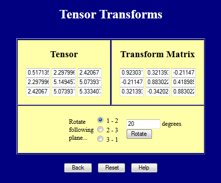
This webpage performs coordinate transforms on 3-D tensors. Try it out.
Coordinate Transforms of 4th Rank Tensors
We will see in the section on Hooke's Law that the stiffness tensor is 4th rank, i.e., 3x3x3x3 (not 4x4). It is written as \(C_{ijkl}\) because it relates any strain component, \(\epsilon_{kl}\), to any stress component, \(\sigma_{ij}\), i.e., \(\sigma_{ij} = C_{ijkl} \epsilon_{kl}\). The coordinate transformation law for the 4th rank stiffness tensor is easily written in tensor notation as\[ C'_{ijkl} = \lambda_{im} \lambda_{jn} \lambda_{ko} \lambda_{lp} C_{mnop} \]
The tensor equation directs how to write the transformation in matrix notation.
\[ {\bf C'} = {\bf Q} \cdot {\bf Q} \cdot {\bf C} \cdot {\bf Q}^T \cdot {\bf Q}^T \]
4th Rank Tensor Transform Example
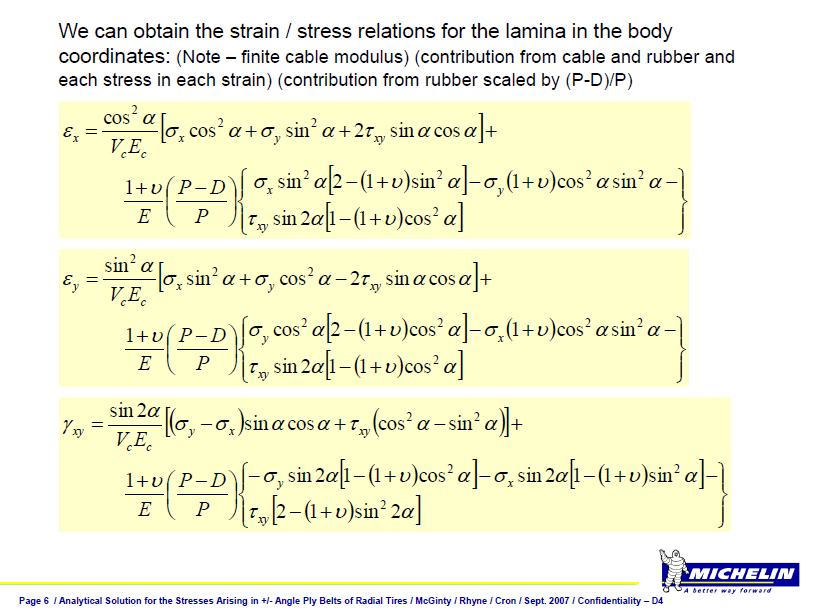
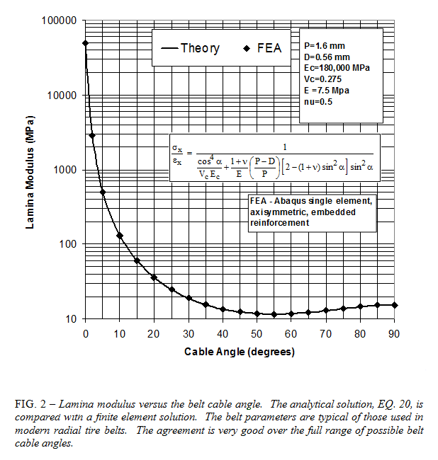
The slides below show the stiffness calculation of a typical single ply steel belt. The angle \(\alpha\) is the rotation of the cables off the longitudinal axis. Note how the equations contain trig functions to the 4th power, This is consistent with the use of four \({\bf Q}\) matrices in the transformation equations.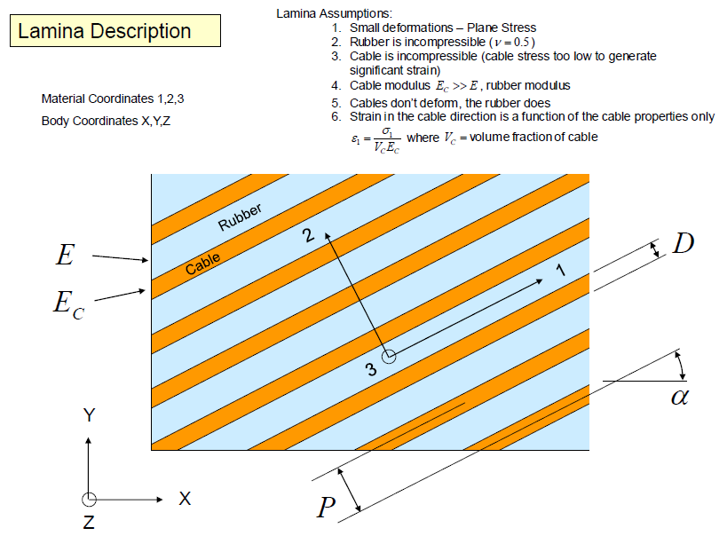
Summary
\[ {\bf v'} = {\bf Q} \cdot {\bf v} \qquad \qquad \text{and} \qquad \qquad v'_i = \lambda_{ij} v_j \]
The coordinate transform of a tensor in matrix and tensor notation is
\[ \boldsymbol{\sigma'} = {\bf Q} \cdot \boldsymbol{\sigma} \cdot {\bf Q}^T \qquad \qquad \text{and} \qquad \qquad \sigma'_{mn} = \lambda_{mi} \lambda_{nj} \sigma_{ij} \]
Note that \({\bf Q}\) and \(\lambda_{ij}\) are the same transformation matrix.
In 2-D, \({\bf Q}\) and \(\lambda_{ij}\) are defined as
\[ {\bf Q} = \left[ \matrix {\;\;\;\cos \theta & \sin \theta \\ -\sin \theta & \cos \theta} \right] \]
which is a special case of the more general 3-D form
\[ {\bf Q} = \left[ \matrix { \cos(x',x) & \cos(x',y) & \cos(x',z) \\ \cos(y',x) & \cos(y',y) & \cos(y',z) \\ \cos(z',x) & \cos(z',y) & \cos(z',z) } \right] \]
where \(\cos(x',x)\) is the direction cosine of the angle between the rotated \(x'\) axis and the reference \(x\) axis.
The coordinate transform of a 4th rank tensor is
\[ {\bf C'} = {\bf Q} \cdot {\bf Q} \cdot {\bf C} \cdot {\bf Q}^T \cdot {\bf Q}^T \]
in matrix notation and
\[ C'_{ijkl} = \lambda_{im} \lambda_{jn} \lambda_{ko} \lambda_{lp} C_{mnop} \]
in tensor notation.